Supra-Kerr 3D Collapse
![]()
Supra-Kerr 3D Collapse
![]()
Introduction
Evolution of Density Profile
Evolution of Lagrangian Matter Tracers
Introduction
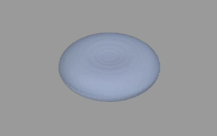
Fig. 1-1 Initial Shape of the Rotating Star
Evolution of the Density Profile
In the meridional clip, the density is plotted on a logarithmic scale normalized to the central density of the star at the current time (Fig 2-1). The clumps first form around t/M = 5.7 (Fig. 2-3). At the final time t/M = 7, the angular momentum satisfies J/M2 = 1.15 which is close to the original value of 1.19 (Fig. 2-5).
Equatorial Plane
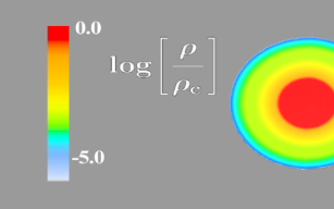 Fig. 2-1 Color code for density profile |
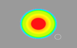 Fig. 2-2 Density profile at t/M = 0 |
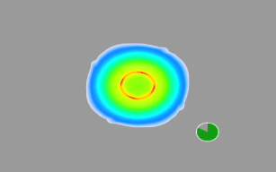 Fig. 2-3 Density profile at t/M = 5.7 |
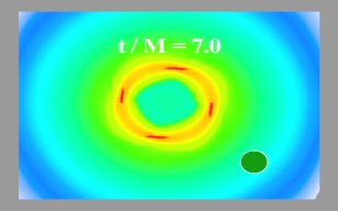 Fig. 2-4 Density profile at t/M = 7.0 |
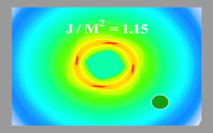 Fig. 2-5 Measurement of the spin parameter at t/M = 7.0 |
**A zoom occurs after the clumps form so visual inspection should not be used to compare sizes.
Evolution of Lagrangian Matter Tracers
In these clips, we track 100,000 Lagrangian matter tracers (particles) that represent fluid elements. The initial distribution of Lagrangian tracers is proportional to the initial mass density. We then calculate the trajectories of the tracers by integrating fluid velocities. The particles are also color-coded according to the density at their current location. Unlike the density profile clip, the densities used to color the particles are normalized to the central density of the star at the initial time. In addition, a separate color coding is used (Fig. 3-1).
Equatorial View
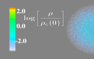 Fig. 3-1 Color code for Lagrangian matter tracers |
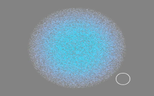 Fig. 3-2 Lagrangian matter tracers at t/M = 0 |
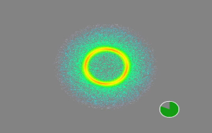 Fig. 3-3 Lagrangian matter tracers at t/M = 5.7 |
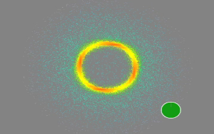 Fig. 3-4 Lagrangian matter tracers at t/M = 7 |
**A zoom occurs after the clumps form so visual inspection should not be used to compare sizes.
Meridional View
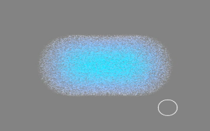 Fig. 3-5 Lagrangian matter tracers at t/M = 0 |
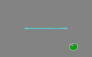 Fig. 3-6 Lagrangian matter tracers at t/M = 5.7 |
 Fig. 3-7 Lagrangian matter tracers at t/M = 7 |
**A zoom occurs after the clumps form so visual inspection should not be used to compare sizes.
last updated 4 December 2014 by aakhan3