Gravitational Waveforms

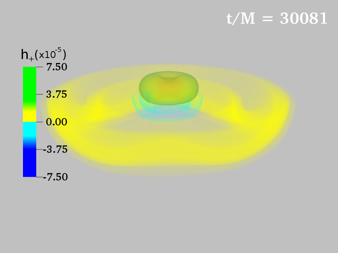
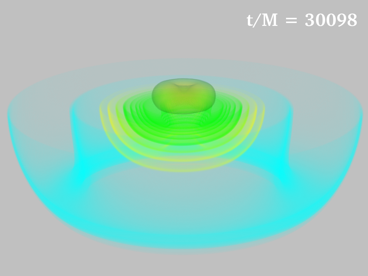
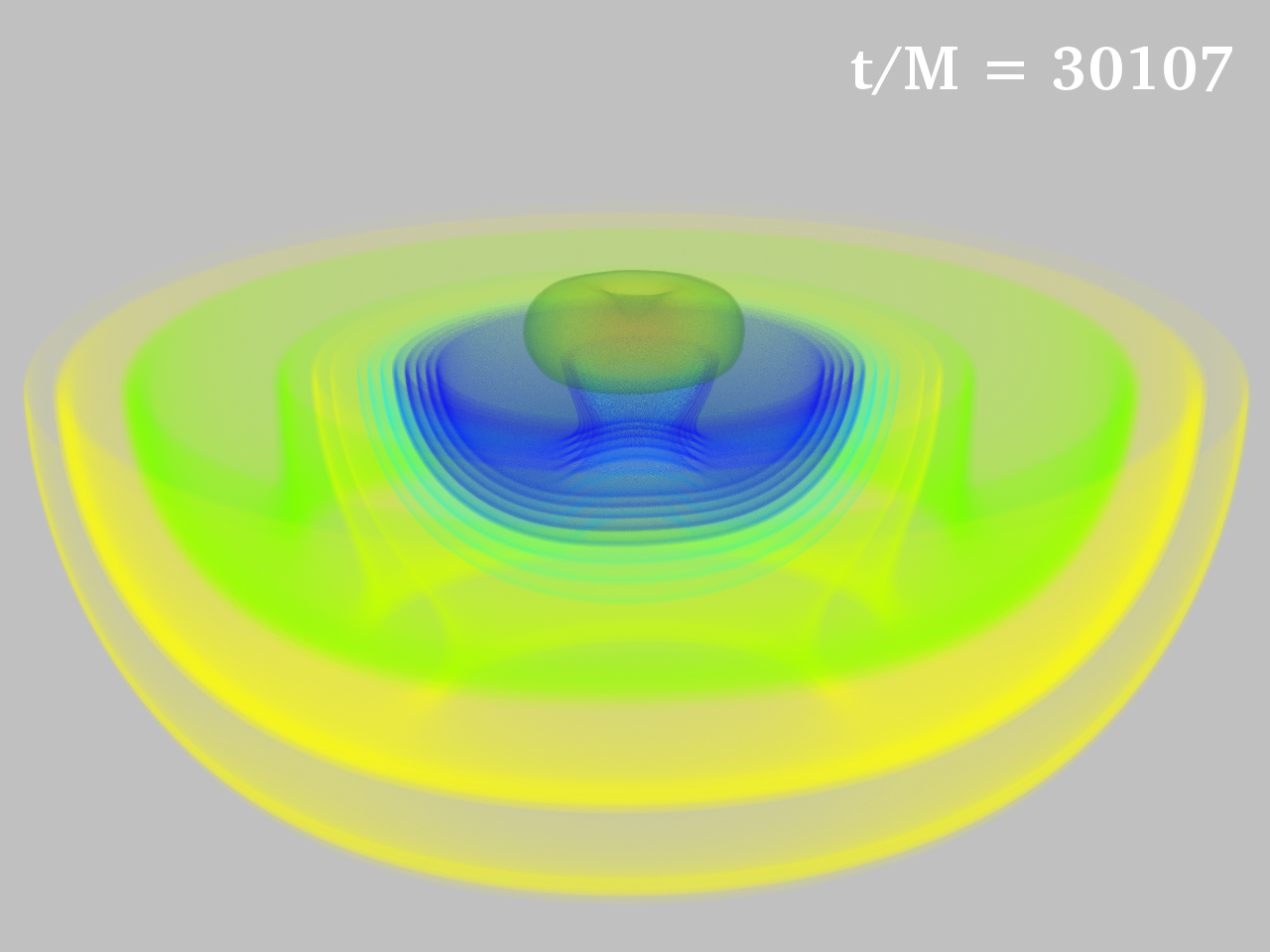
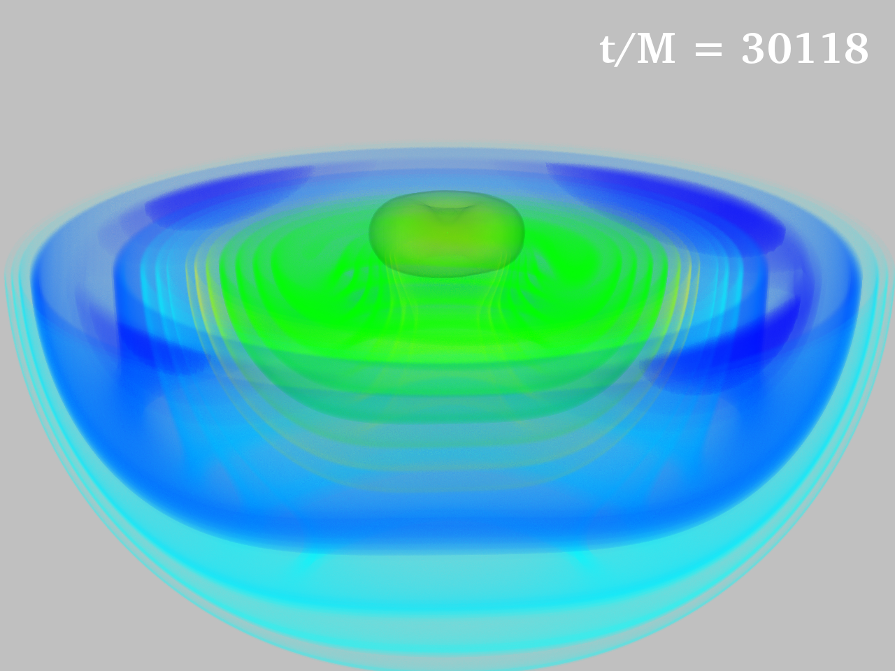
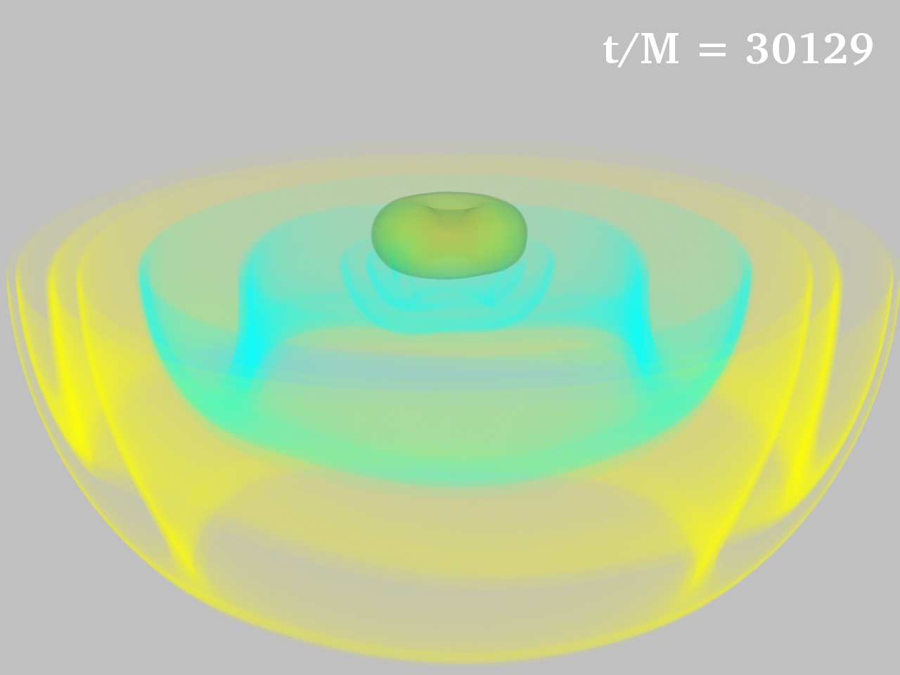
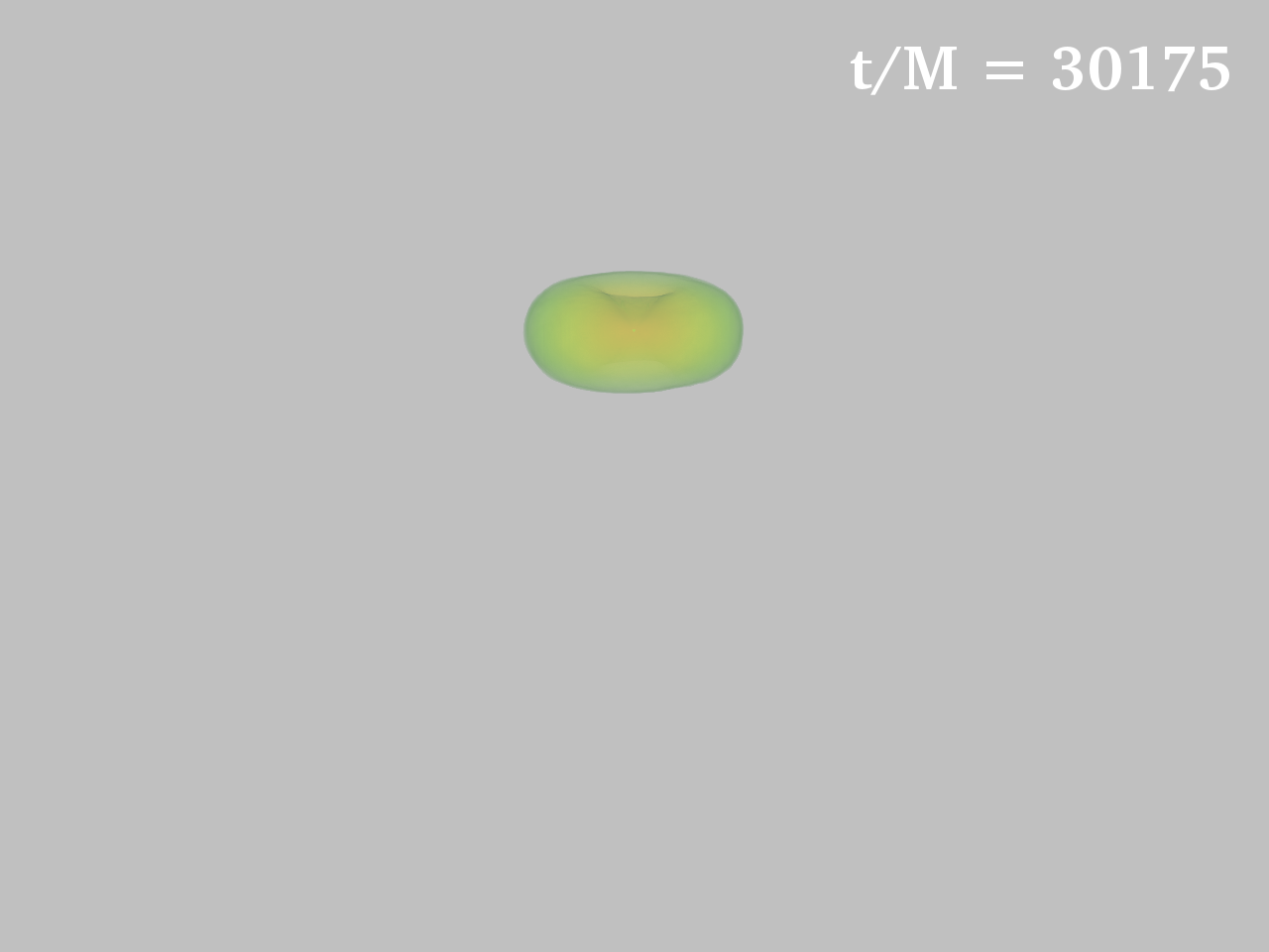
The gravitational wavestrain from SMS collapse may be separated into two qualitatively different phases: the collapsing phase and the BH ringdown. During the early collapsing phase, the gravitational wave has smaller, growing intensity and lower frequency. As the matter source becomes denser, the wave intensity increases and right before the BH forms, the intensity reaches its peak. Once the BH forms, ringdown radiation is emitted as the distorted BH settles down to Kerr-like equilibrium (Note: Only in the case of a vacuum spacetime does the spinning BH obey the exact Kerr solution). The BHs formed here are surrounded by gaseous disks with $M_{\text{disk}} \sim 0.1 M_{\text{BH}} $. Since the collapse is nearly axisymmetric, the dominant amplitude is the h+ polarization, with nearly zero h× polarization. The plot for h+ is shown below, and applies to a $\Gamma = 4/3$ equation of state (pure radiation).
Waveform Analysis
Figure 2-1 shows the real part of the quadrupole mode with the $l = 2$, $m = 0$ component of the Weyl scalar $\Psi_{2,0}$ for the four cases in this project. No significant differences of wavelength exist among all four cases. However, there are differences between the amplitudes of each case.
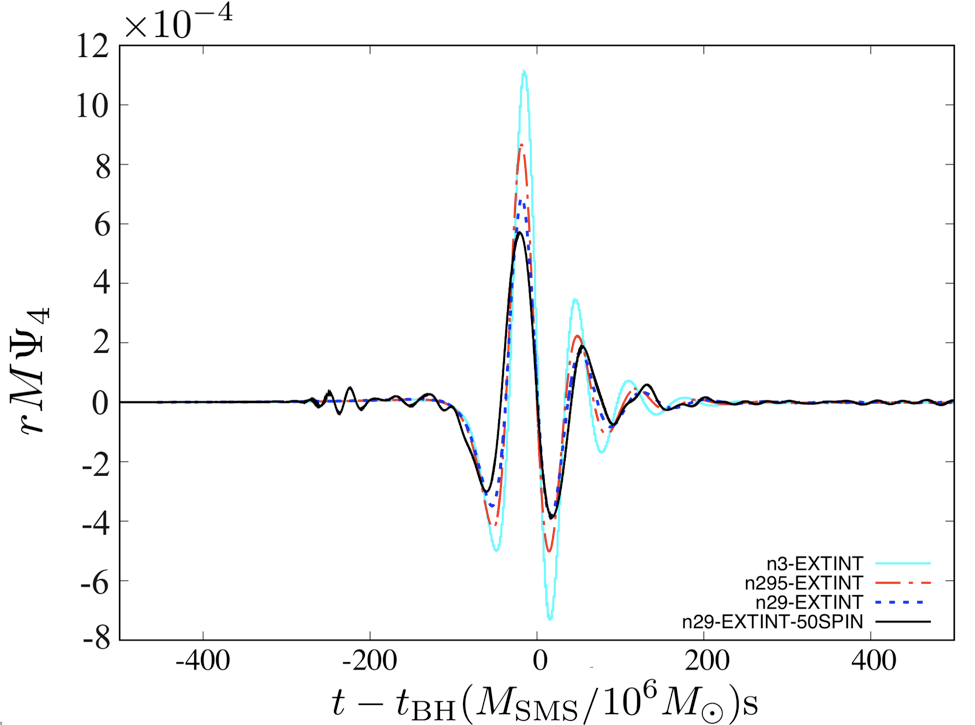
Fig. 2-1: Real part of Weyl scalar $\Psi_{2,0}$ for $4$ cases as a function of retarded time. Gravitational waves are extracted at r = $100.6$ M. The time has been shifted by the BH-formation time $t_{BH}$ for each case respectively.
For a SMBH with mass $\sim 10^6 M_{\odot}$, the frequency is located in the most sensitive band of LISA for $z \lesssim 7$. To confirm detectability, we calculate the strain amplitude $|h(f)| = (h(f)_+^2 + h(f)_{\times}^2)^{1/2}$ and compare with the sensitivity curve of current GW detectors. Fig. 2-2 shows the Fourier spectrum of strain times frequency $|h(f)|f$ versus frequency for three cases at redshift $z=1$ and Case A at $z =$ 2 and 3 alongside the characteristic strain amplitude, $S(f)\,f^{1/2}$, where $S(f)$ is the linear spectral density, from two different modes of LISA. Both modes have 4 laser links and arm length $L = 5 \times 10^6$ km with one having an optimistically functioning LISA Pathfinder (N2) and the other 10 times lower (N1). As expected from the Weyl scalar, waveforms of the three cases overlap closely at the same redshift. With $M = 10^{6} M_{\odot}$, the peak strain at $z=1$ is:
$$ h \approx 9.2 \times 10^{-21} \left(\frac{M}{10^6 M_{\odot}}\right) \left(\frac{6.8 \text{ Gpc}}{D_L}\right) $$
where $D_L = 6.8$ Gpc, corresponding to redshift $z=1$ in a $\Lambda\textrm{CDM}$ cosmology model with $H_0 = 67.6 \text{ km s}^{-1} \text{Mpc}^{-1}$ and $\Omega_{M} = 0.311$. In addition, the plot shows that the peak strain is located near the most sensitive frequency range of LISA. For the N1 configuration, the $\textrm{SNR}$ is about 5 at $z=1$. If the sensitivity of LISA is enhanced to that of LISA project (N2), the observation of GW signals for a similar object as far as $z=3$ is possible with $\textrm{SNR} \gtrsim 10$. Due to the extremely low gas metalicity, a SMS is unlikely to form for $z \lesssim 2.5$. Hence, a GW detector as sensitive as LISA is required to detect such signals.
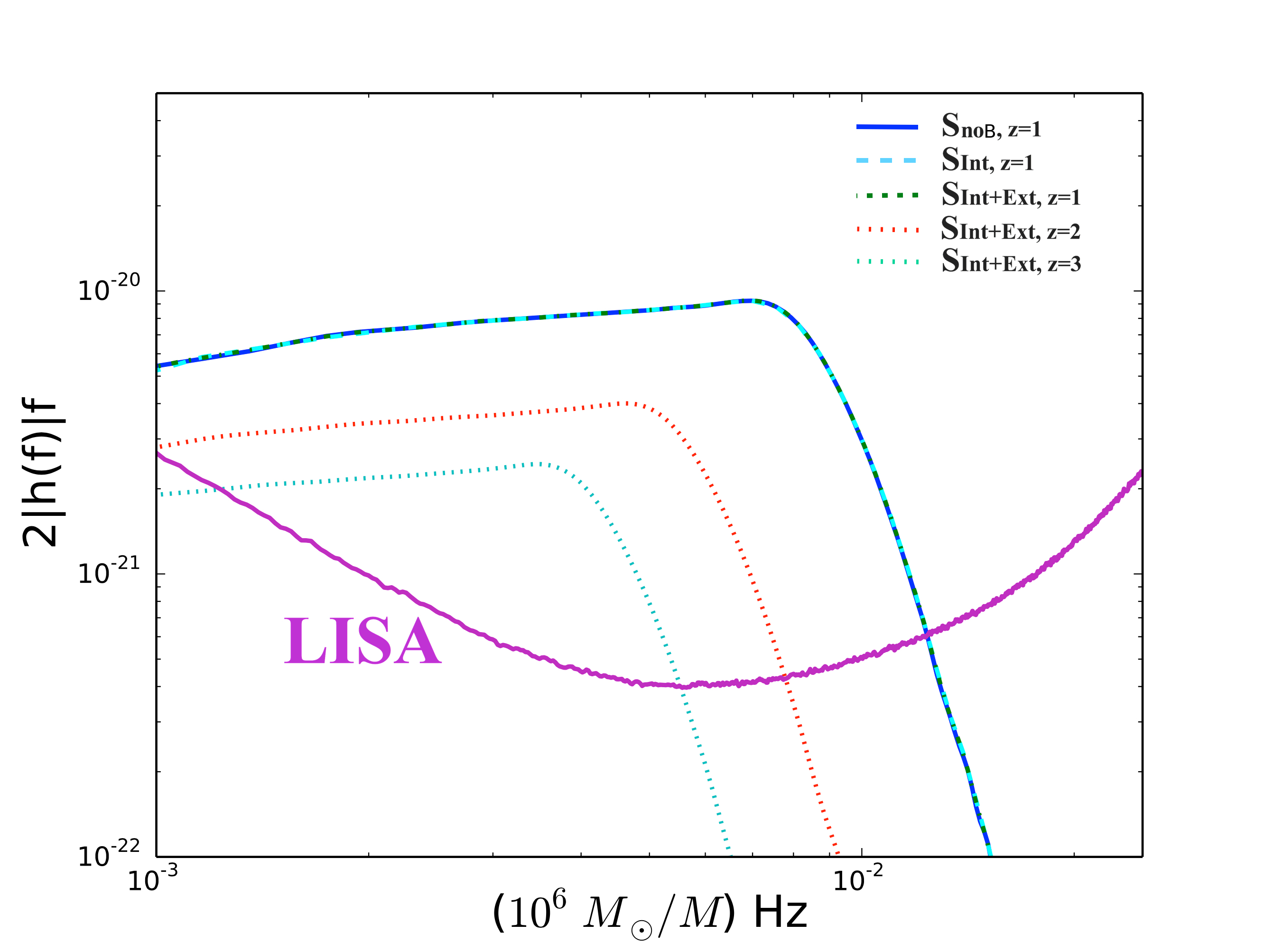
Fig. 2-2: $2|h(f)|f$ vs. frequency diagram for collapse models. The upper (3 overlapped), middle and lower curves denote the signal strength from $z =$ 1, 2, and 3, respectively. The bottom curve is the characteristic strain amplitudes of LISA. |
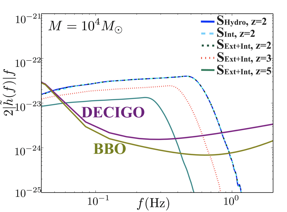
Fig. 2-3: $2|\tilde{h}(f)|f$ vs. frequency diagram for collapse models. The upper (3 overlapped), middle and lower curves denote the signal strength from $z =$ 2, 3, and 5, respectively. The 2 bottom curves are the characteristic strain amplitudes of DECIGO and BBO. |
In figures 2-2 and 2-3:
• SnoB and SHydro denote cases with the same $\Gamma = 4/3$ equation of state as Case A, but with zero B-field.
• SInt denotes cases with the same equation of state as Case A, but with B-field confined inside the SMS.
• SInt+Ext and SExt+Int denote Case A.