Gravitational Waveform Comparison

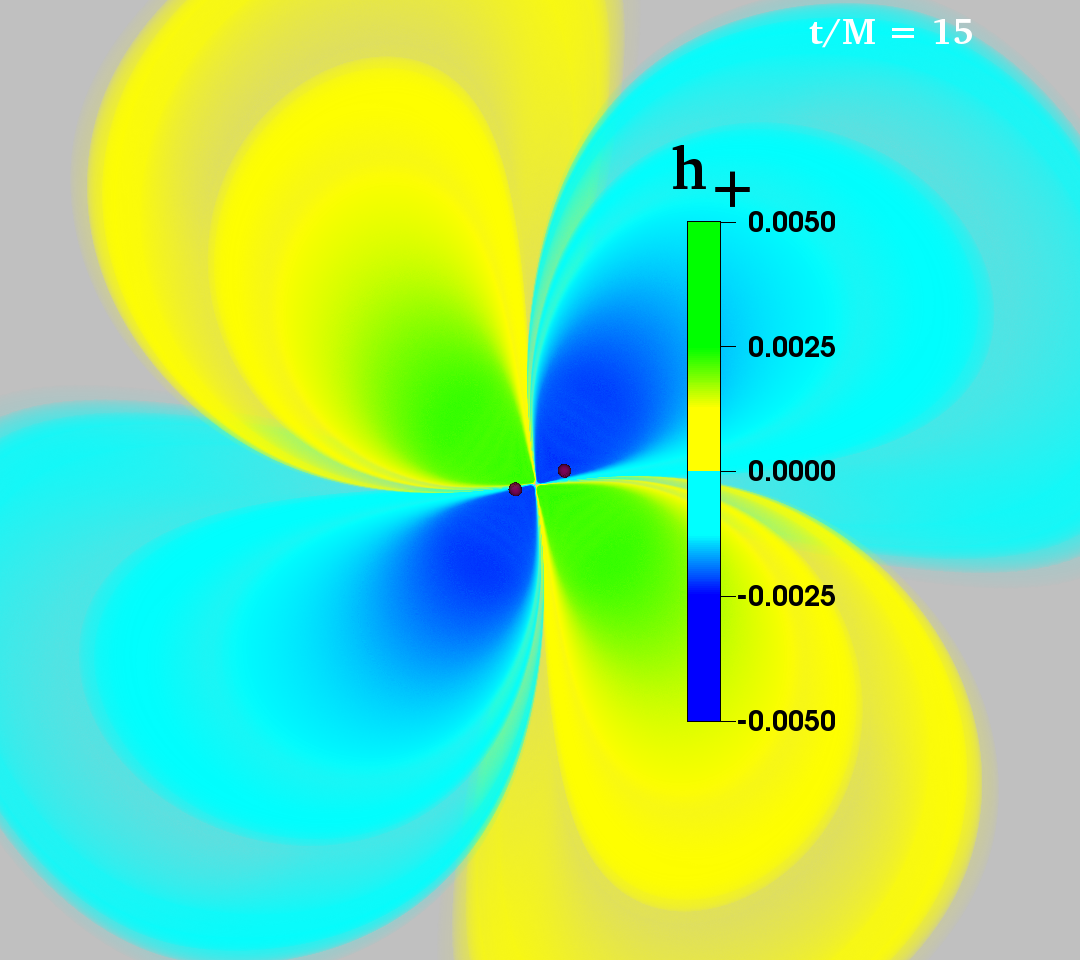 Fig. 1-1: t/M = 15 |
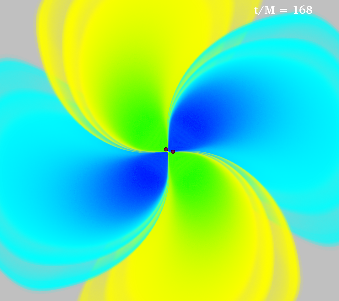 Fig. 1-2: t/M = 168 |
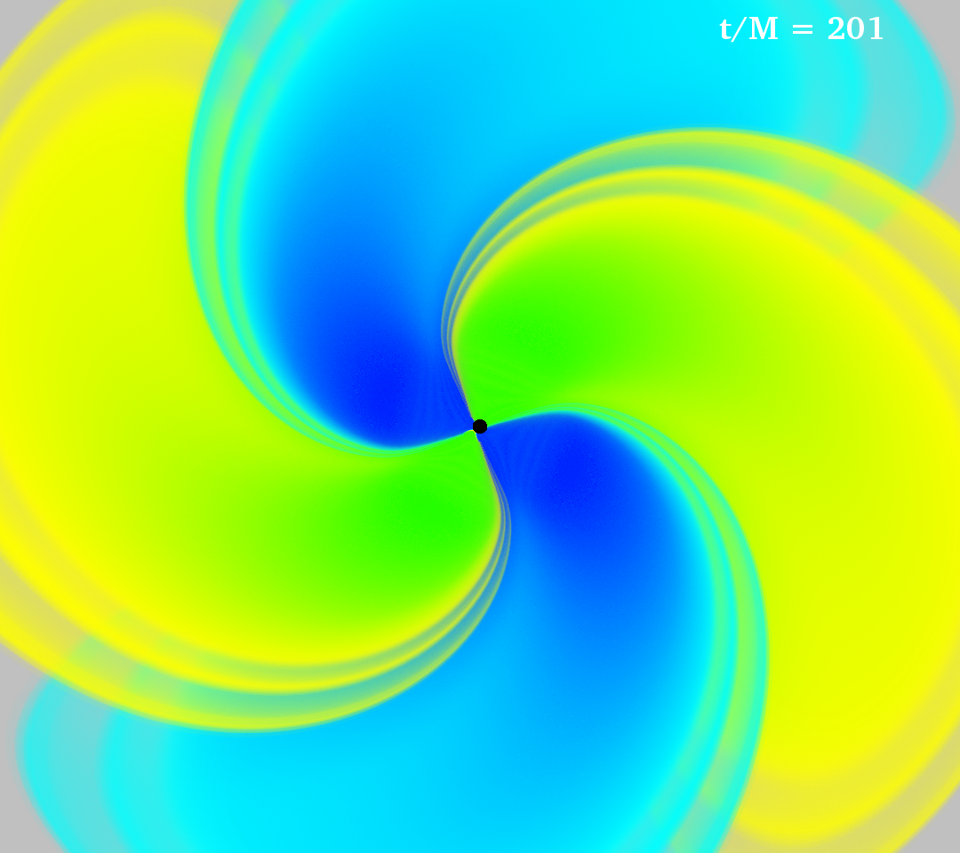 Fig. 1-3: t/M = 201 |
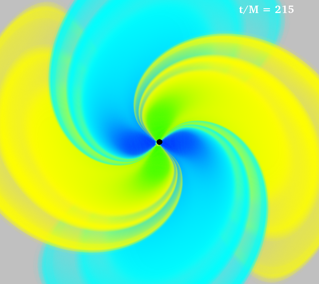 Fig. 1-4: t/M = 215 |
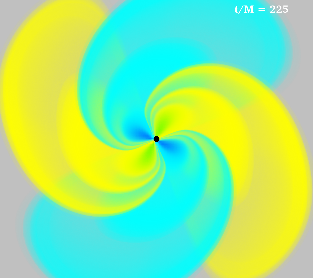 Fig. 1-5: t/M = 225 |
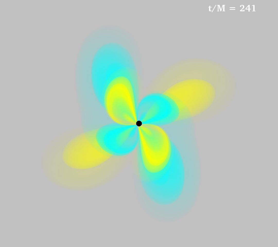 Fig. 1-6: t/M = 241 |
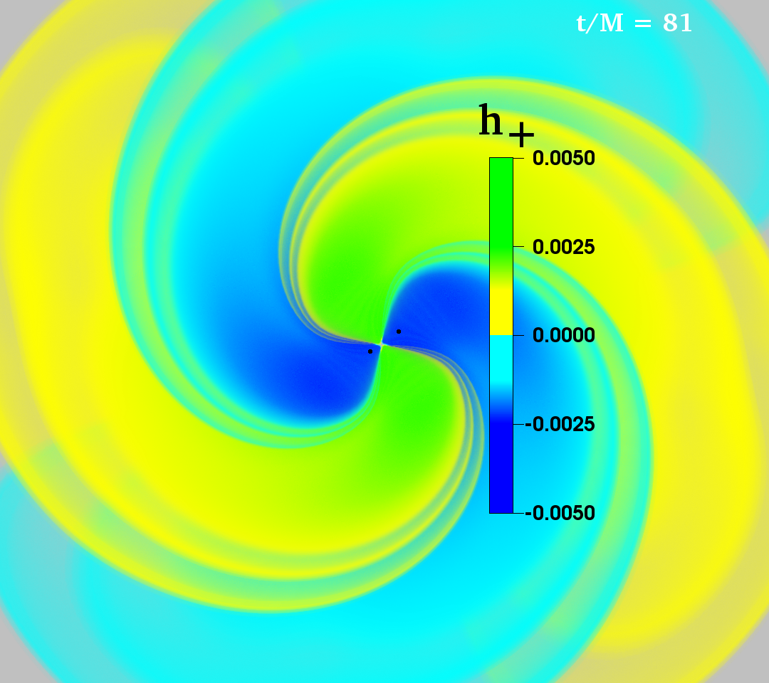 Fig. 2-1: t/M = 81 |
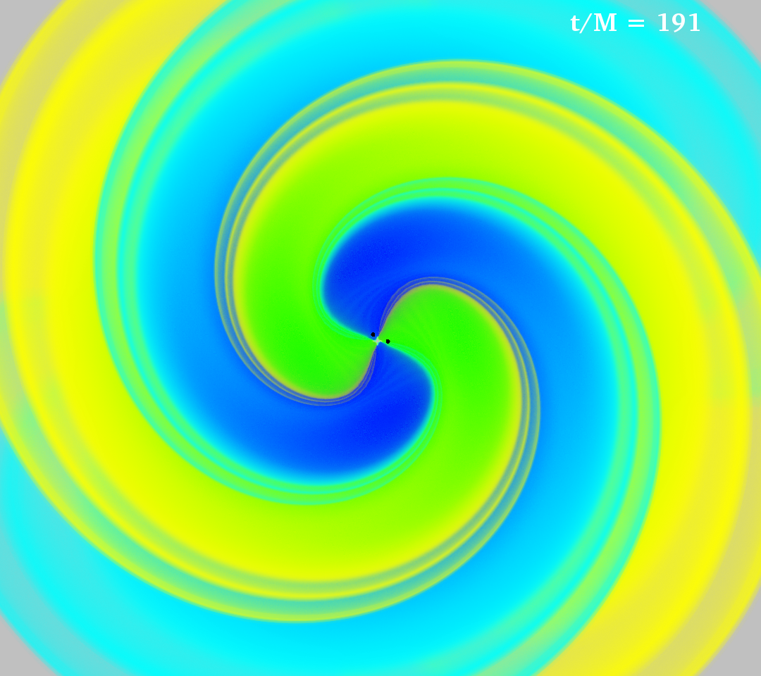 Fig. 2-2: t/M = 191 |
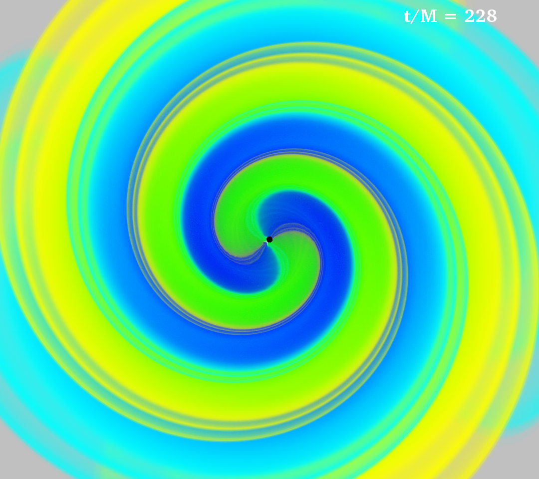 Fig. 2-3: t/M = 228 |
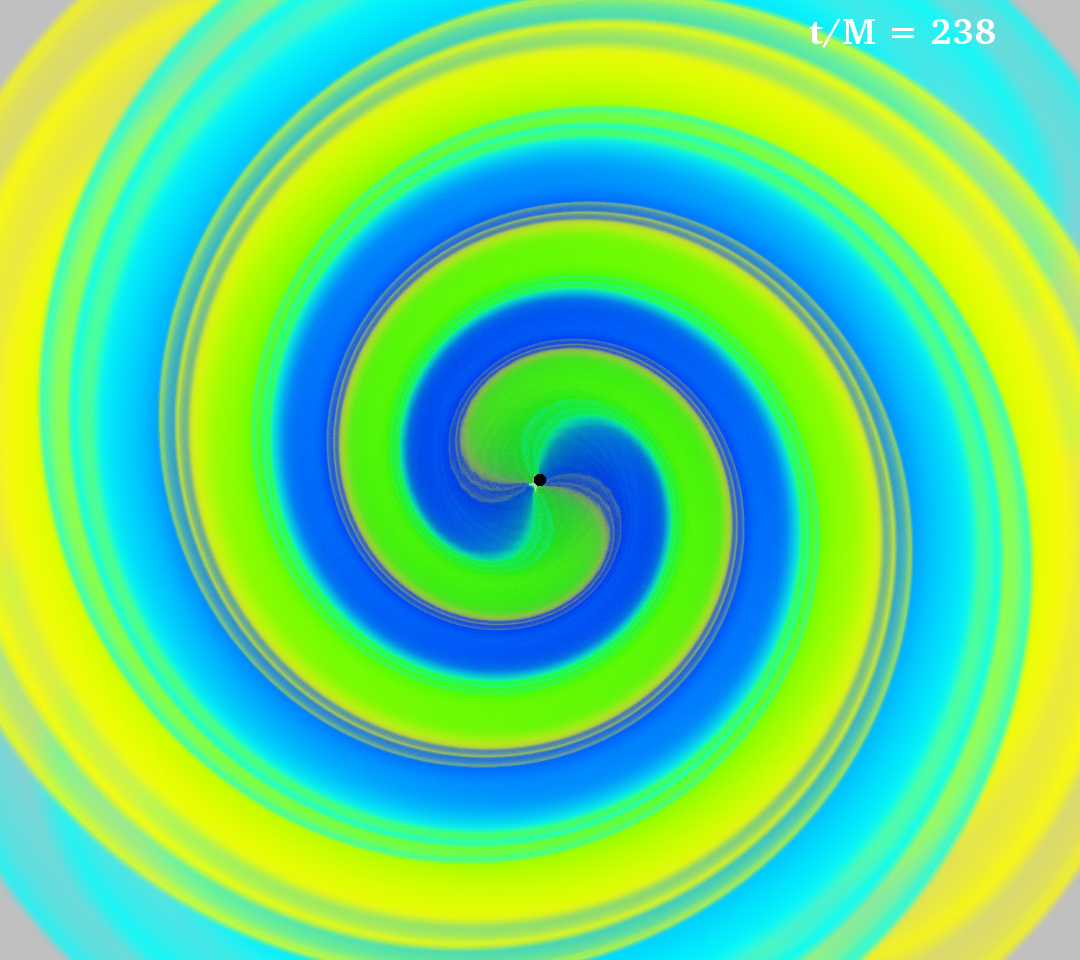 Fig. 2-4: t/M = 238 |
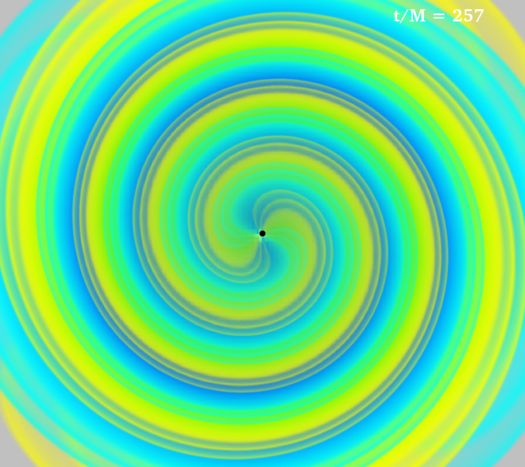 Fig. 2-5: t/M = 257 |
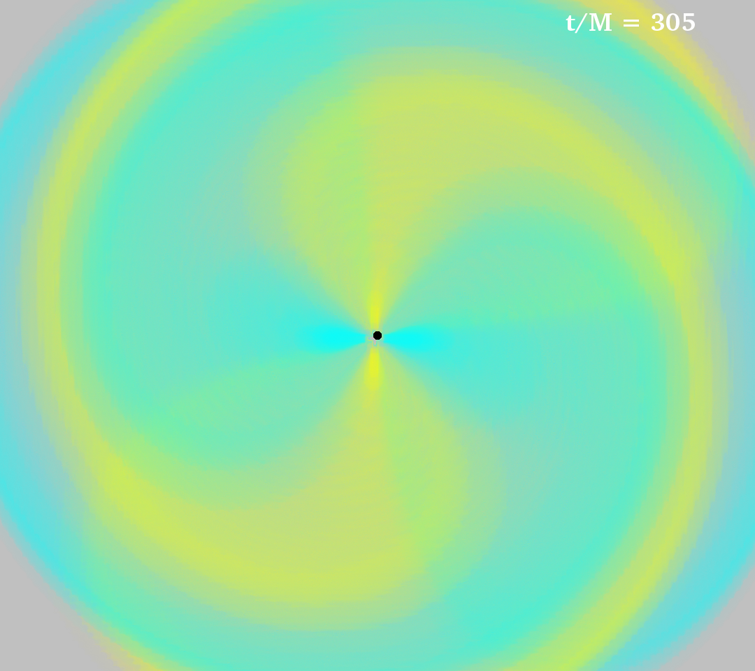 Fig. 2-6: t/M = 305 |
The early inspiral of both the NSNS and BHBH are very similar until tidal interactions begin at $t/M \sim 130$. The angular velocity of the BHBH binary is smaller than the NSNS binary at any given time which leads to a delayed merger of the BHBH binary. We conclude that, when the results are extrapolated to infinite resolution, the largest phase difference between the NSNS and BHBH binary is 4.5 rads within the $[0.6, 1.0] KHz$ bandwidth. Our maximally compact stars yield a minimal but measurable phase difference. To quantify the difference in power spectral density of the two binaries, we computed the match function $$\mathcal{M} = \underset{(\phi_c,t_c)}{{\rm max}} \frac{(\tilde{h}_1|\tilde{h}_2(\phi_c,t_c))}{\sqrt{(\tilde{h}_1|\tilde{h}_1)(\tilde{h}_2|\tilde{h}_2)}}$$ where the maximization is taken over a large set of phase shifts $\phi_c$ and time shifts $t_c$. Here $(\tilde{h}_1|\tilde{h}_2)$ denotes the standard noise-weighted inner product. For both NSNS binary resolutions, we find $\mathcal{M} = 0.998$ which implies that with current detectors (e.g. aLIGO/Virgo) the waveforms are distinguishable for a signal-to-noise ratio of, e.g., 25, comparable to GW150914. However, uncertainties in the orbital parameters will likely prevent these detectors from distinguishing these compact, massive NS binaries from BH binaries.
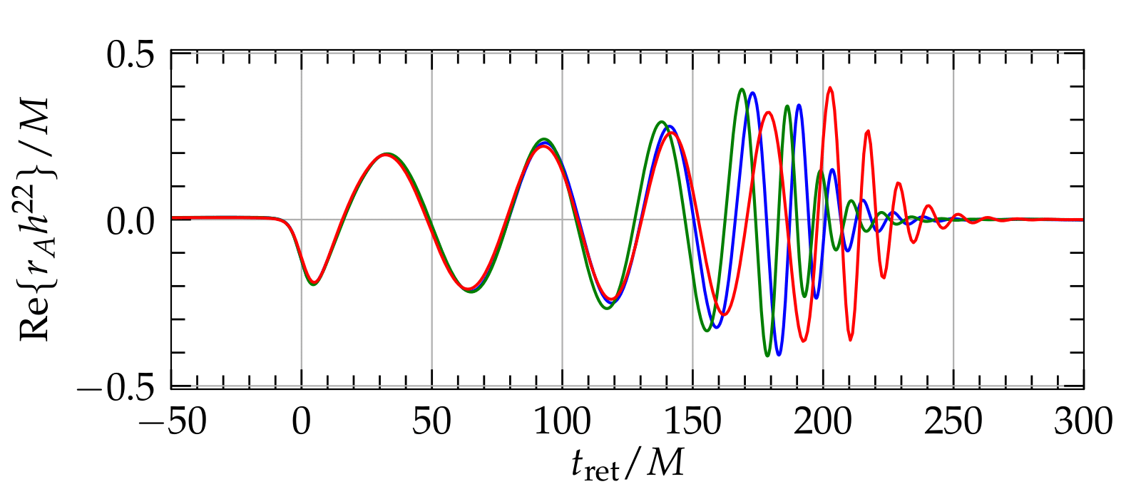 Fig. 3-1: Strain vs retarded time for the $(\ell = 2, m = 2)$ dominant mode |
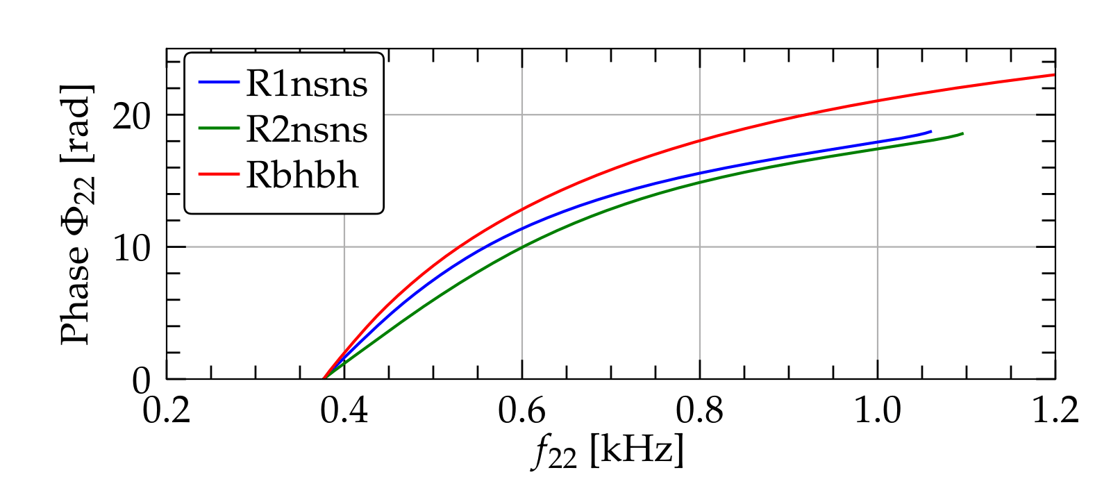 Fig. 3-2: The phase $\Phi_{22}(t)$ of the strain up until its maximum vs the GW frequency |
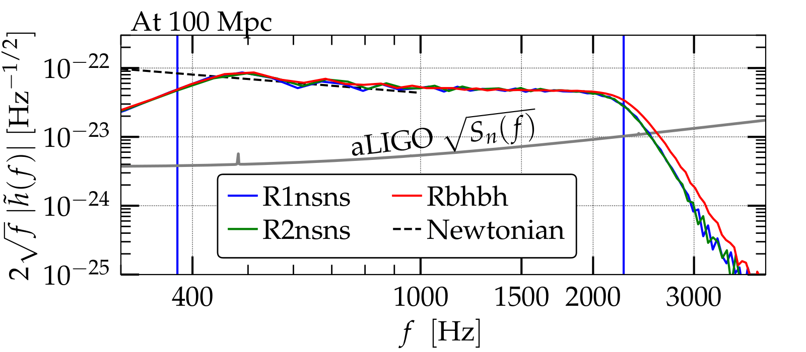 Fig. 3-3: Fourier spectra of numerical waveforms |