NSNS vs BHBH Evolution

The evolution of the NSNS system is depicted below where isocontours of density $\rho_0=2.26\times 10^{13}\ {\rm gr/cm^3} = \rho_0^{\rm max}(0)/22.4$ are plotted at various times during the inspiral. This isocontour corresponds to the density at a radial distance $0.998 R_x(0)$ measured from the maximum density point in the NSs; therefore it is an accurate representation of the surface of the star. In accordance with the (PN) prediction the binary performs approximately $\sim 1.7$ orbits, with the two stars starting as two spherical configurations to high accuracy.
Tidal distortion becomes evident only after $1.5$ orbits when $t/M\approx 170$. Shortly afterwards (less than a quarter of an orbit) merger begins with no cusp formation. The surface remains intact up until the merging of the two NSs at $t/M=180$ where they actually touch. Immediately thereafter the remnant collapses, at $t/M\sim 183$ when the structure still has a clear dumbbell shape as in the snapshot in Fig. 1-4. The apparent horizon immediately after collapse has a spherical shape but settles as a prolate configuration at the end of the simulation. This is simply a gauge effect caused by the NSNS moving puncture coordinates. The ratio of polar to equatorial circumferences of the horizon asymptotes to $\sim 0.89$ $<$ $1$, in agreement with the Kerr value for a spinning BH with $a/M_{bh} = J_{bh}/M_{bh}^2 = 0.71$.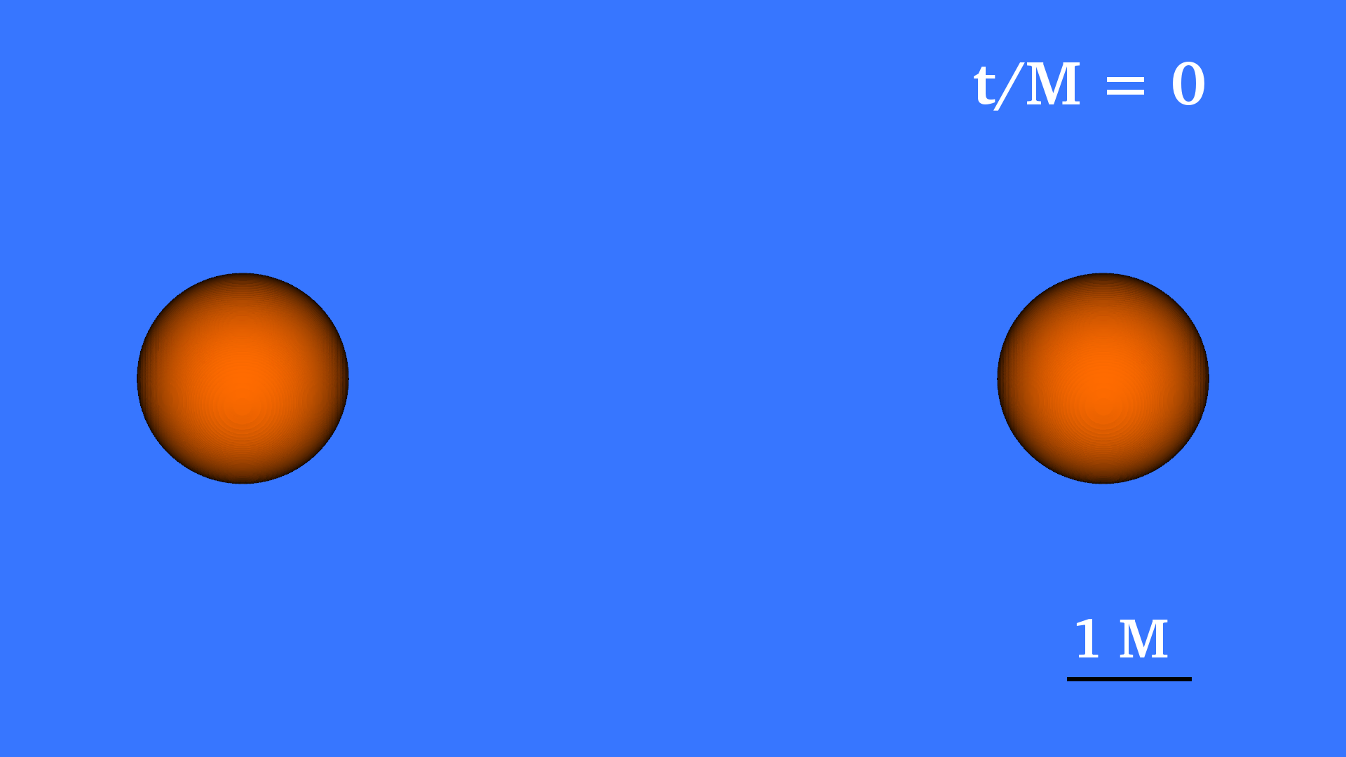 Fig. 1-1: Density isocontour |
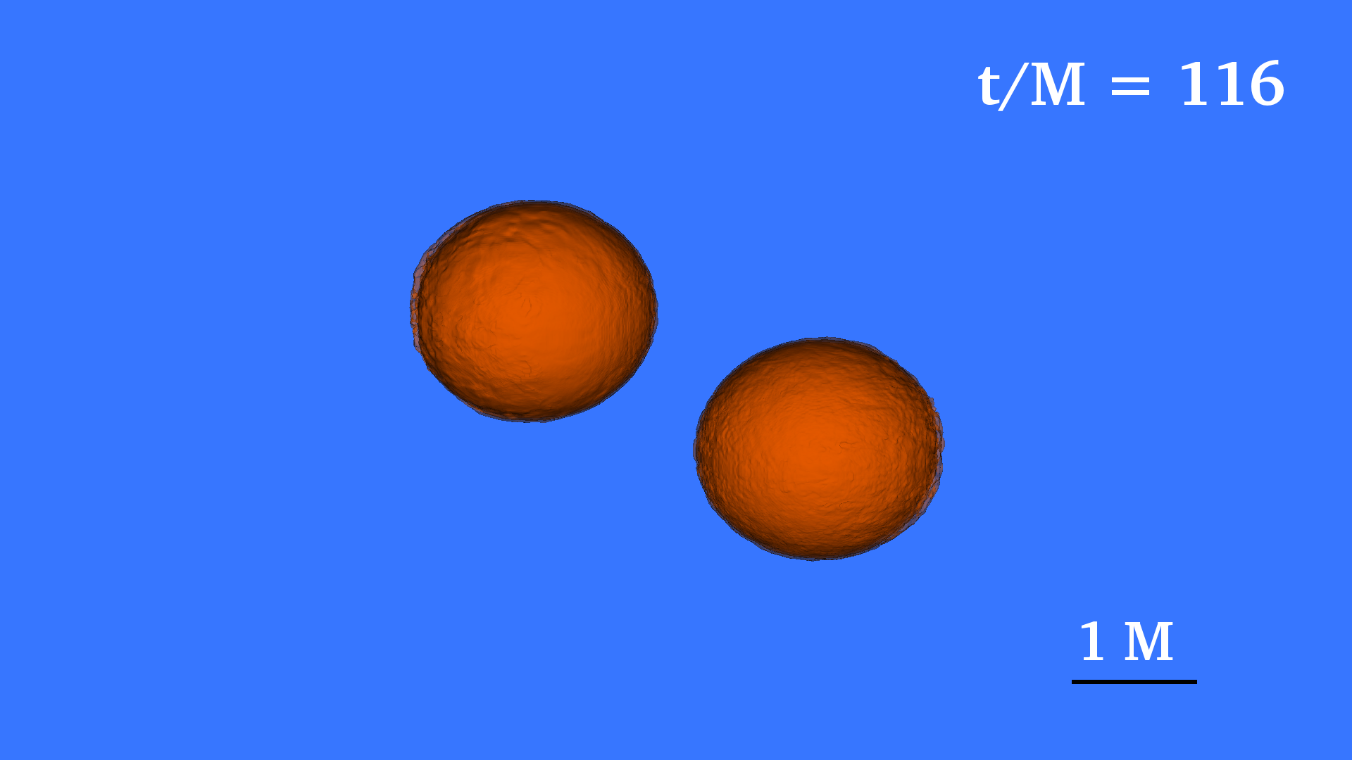 Fig. 1-2: Density isocontour |
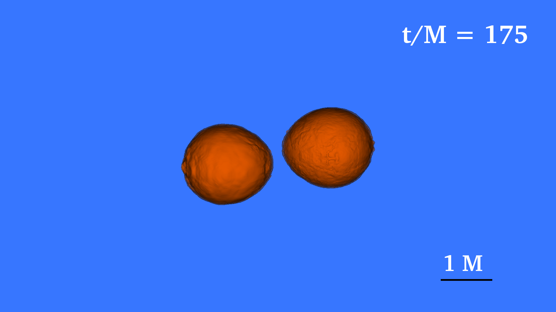 Fig. 1-3: Density isocontour |
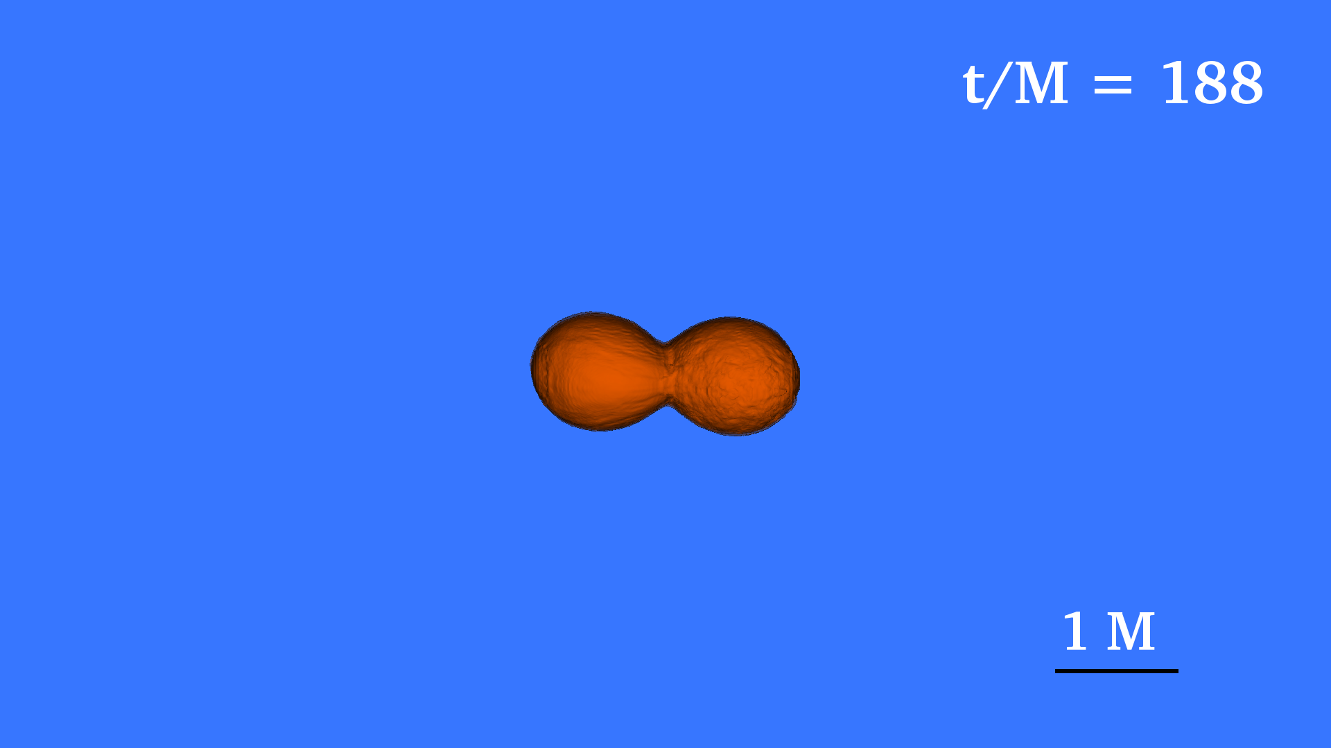 Fig. 1-4: Density isocontour |
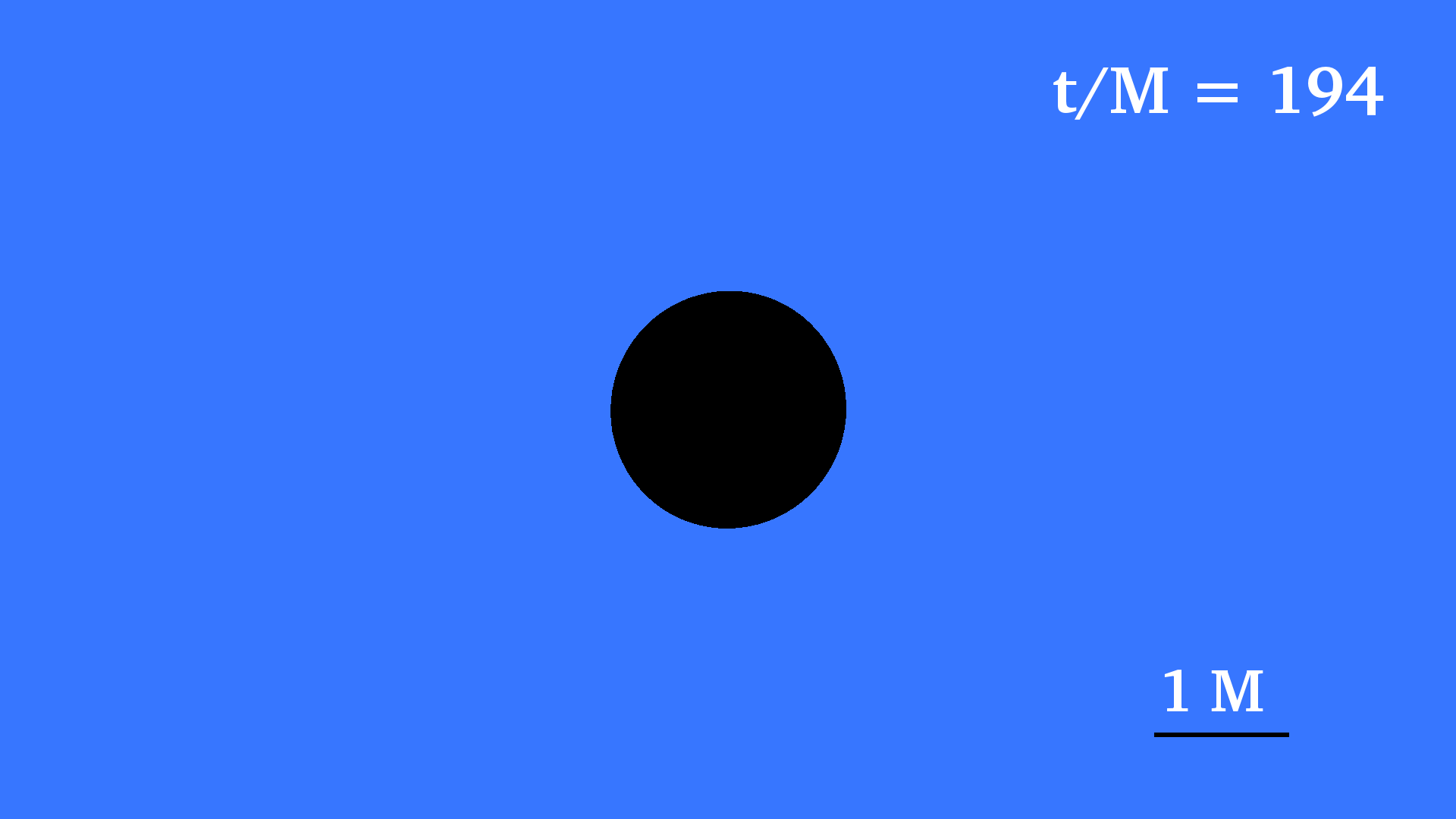 Fig. 1-5: NSNS remnant |
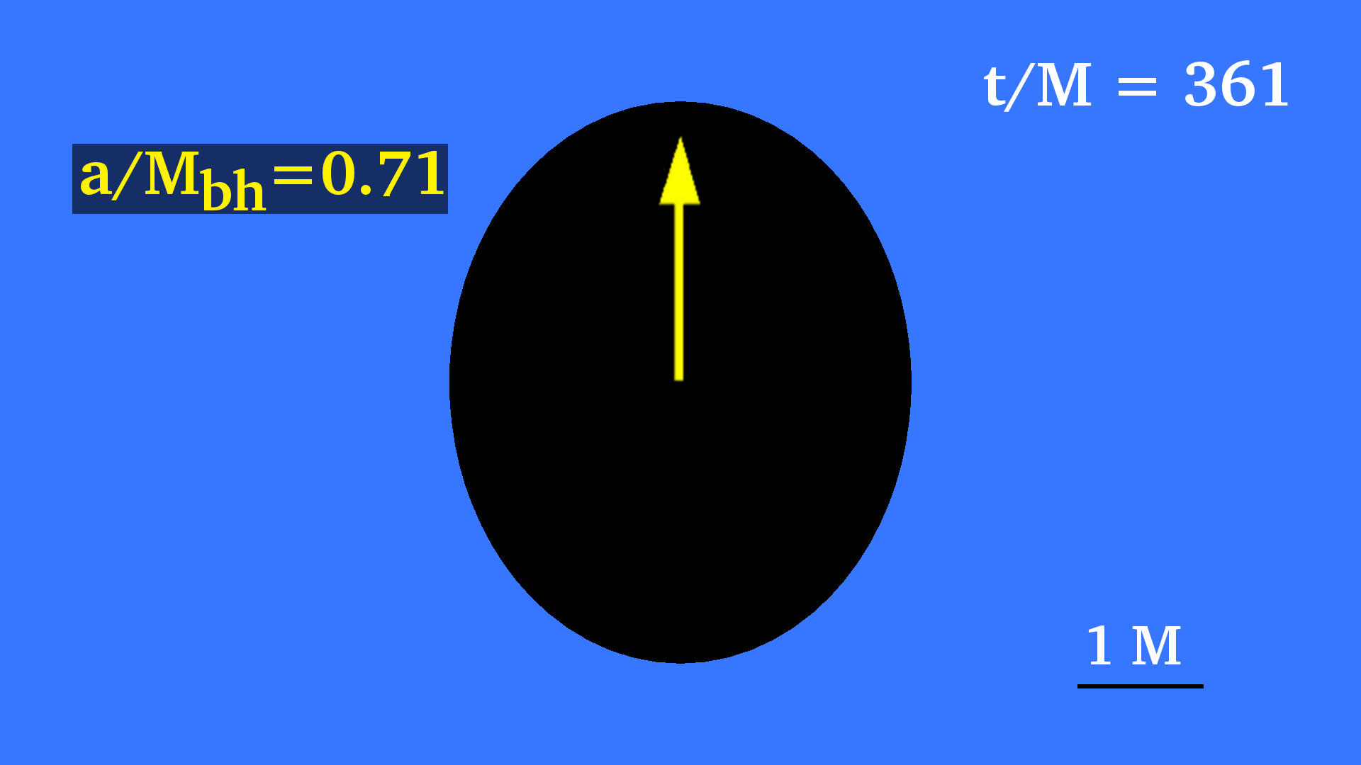 Fig. 1-6: NSNS remnant |
The BHBH system evolves similarly to the NSNS system. However, the NSNS system merges earlier than the BHBH system.
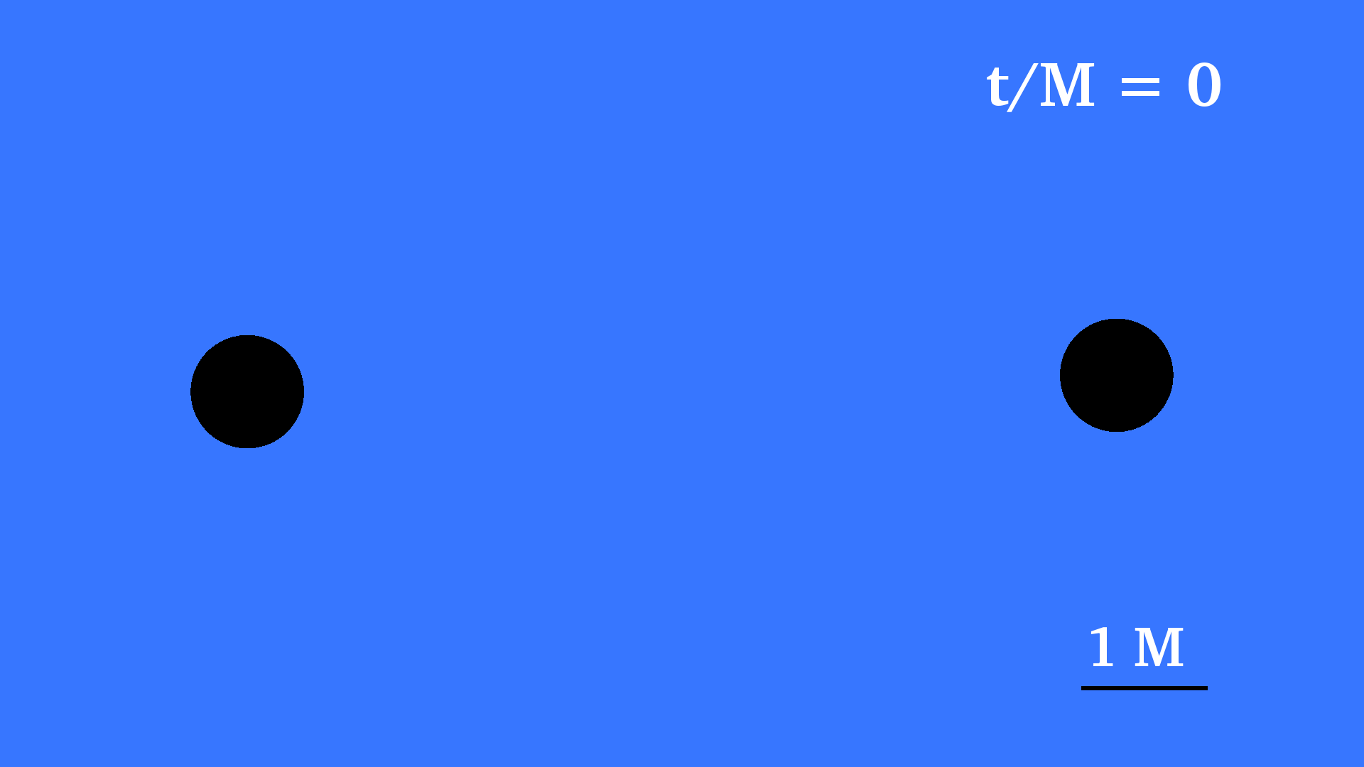 Fig. 2-1: BHBH evolution |
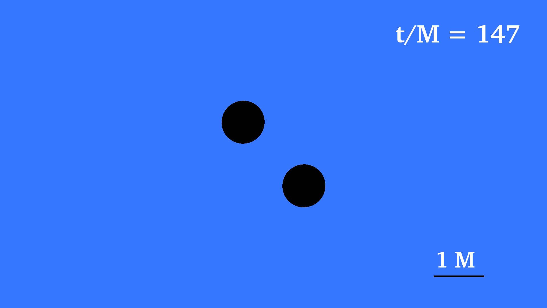 Fig. 2-2: BHBH evolution |
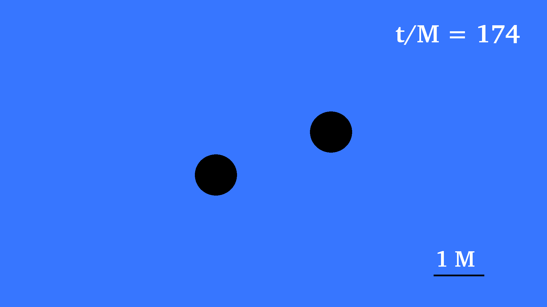 Fig. 2-3: BHBH evolution |
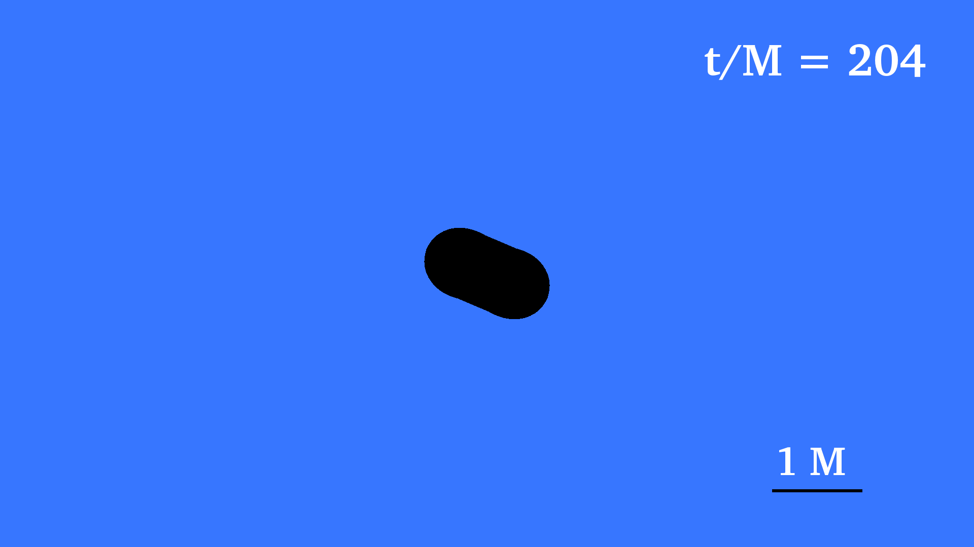 Fig. 2-4: BHBH evolution |
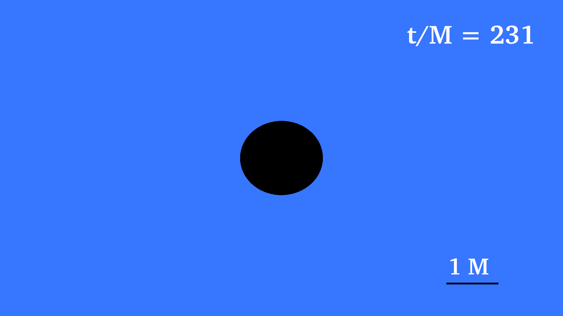 Fig. 2-5: BHBH evolution |
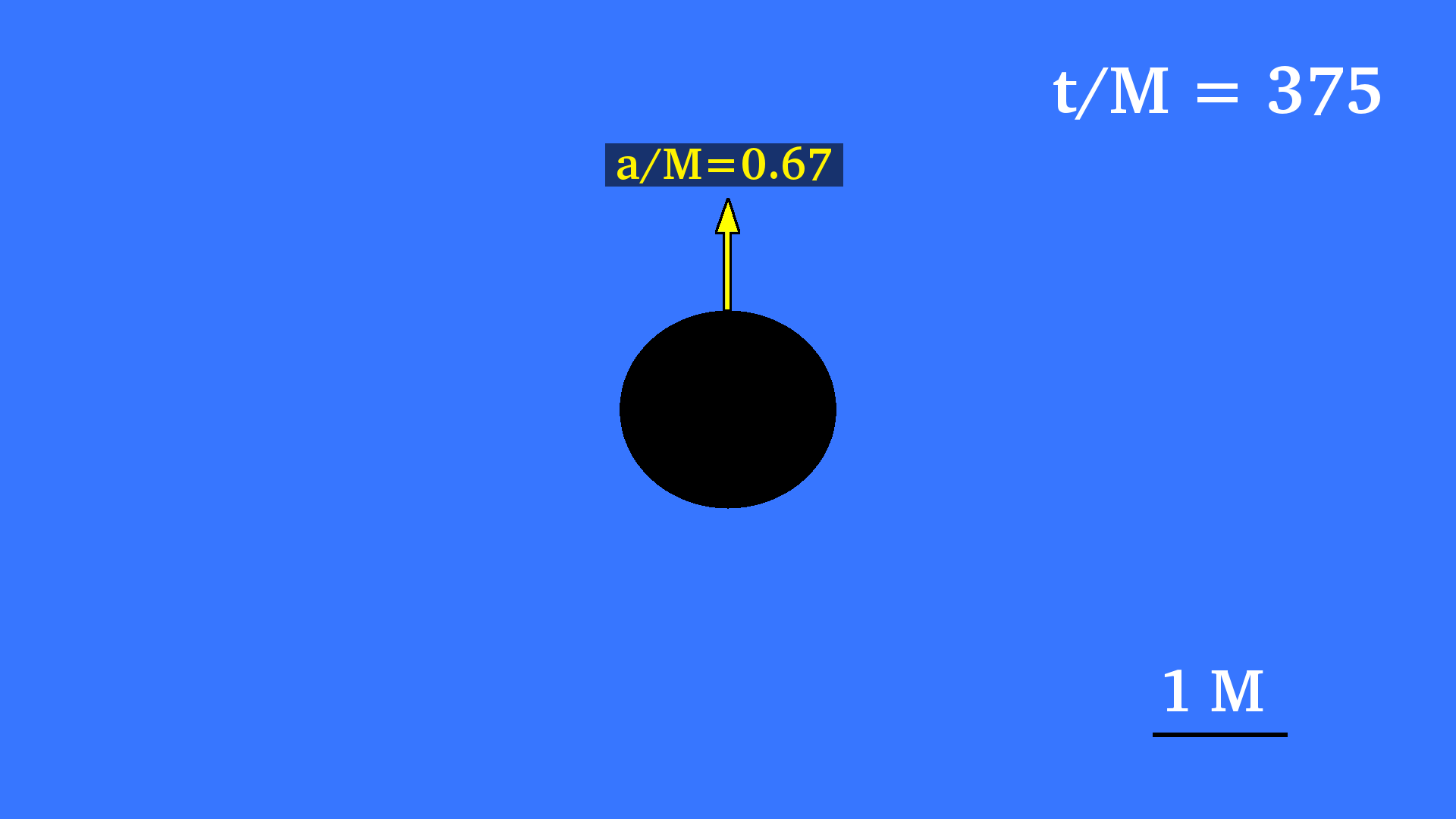 Fig. 2-6: BHBH evolution |
We use two methods to diagnose the spin of the remnant BHs. First, we calculate $a/M_{bh} = J_{bh}/M_{bh}^2$ using the isolated horizon formalism. Here we use R1nsns and Rbhbh for the NSNS and BHBH runs respectively. Second, we start from the expression $L_p/L_e = 4\sqrt{r_+^2 + a^2}E \left (\frac{a^2}{r_+^2 + a^2} \right) $ which is the ratio of proper polar horizon circumference, $L_p$, to the equatorial one, $L_e$, in Kerr spacetime. Here $E(x)$ is the complete elliptic integral of the second kind. The above expression can be approxmiated to $$ \frac{L_p}{L_e} \approx \frac{\left (\sqrt{1-(a/M_{\rm bh})^2}+1.55 \right)}{2.55} $$ which allows us to get estimates for $a/M_{bh}$. After calculating $L_p/L_e$ directly from the metric, we computed estimates for $a/M_{bh}$ which appear in the figure below. The two spin diagnostics agree to a level of $\sim 1.5\%$ for both binaries, while the spin of the BHBH binary remnant differs from the one of the NSNS binary remnant by $\sim 4\%$ with the NSNS remnant BH having higher spin.
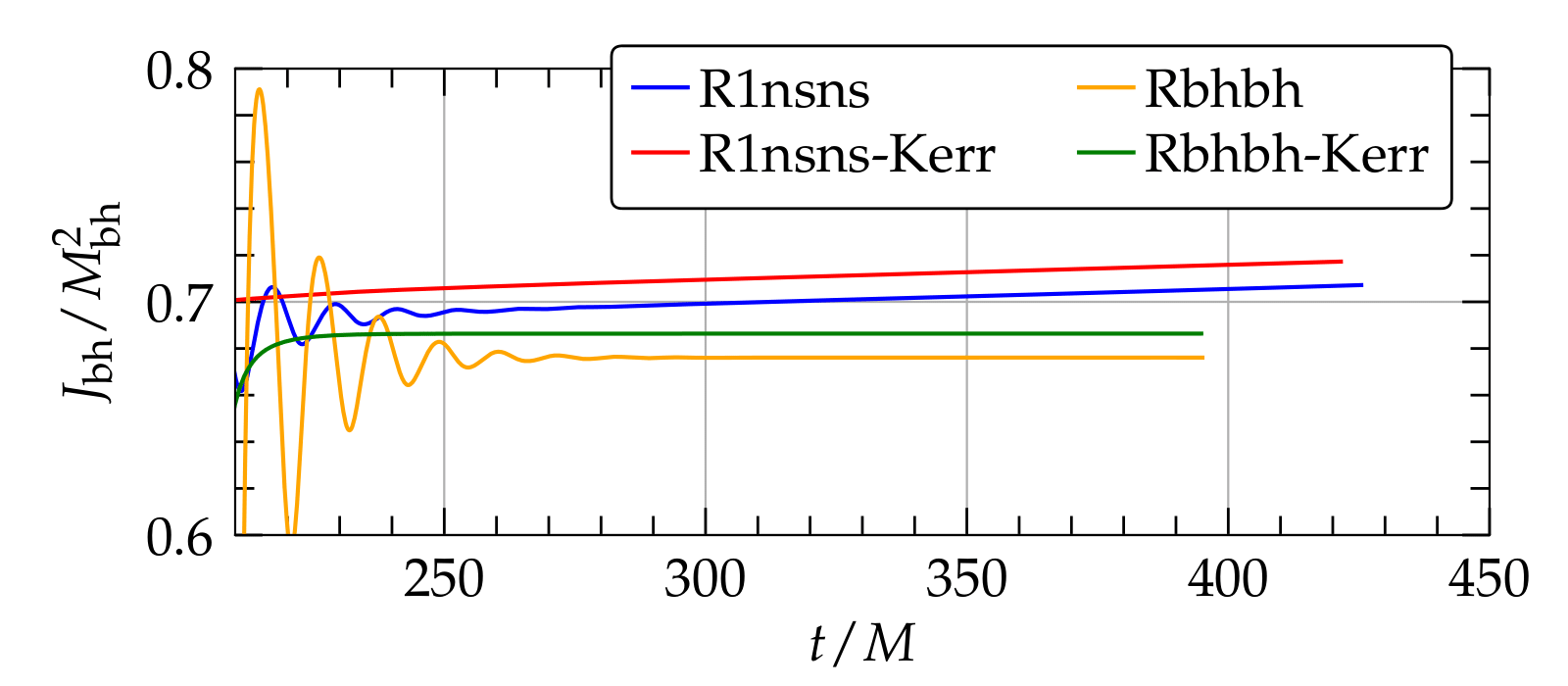 Fig. 3-1: Spin of the remnant BHs |
Although the mode frequencies $\omega_{\ell m}$ of the GW signal during inspiral and merger are described by complicated functions of time, during ringdown the GW signal can be described with high accuracy as a simple superposition of damped sinusoids characterized by three indices: the two spherical harmonic indices $\ell,\ m$ and a third overtone index, $n=0,1,\ldots$, which here we assume to be the fundamental one $n=0$. As a consequence of the no-hair theorem, all dimensionless mode frequencies, $M_{\rm bh}\omega_{\ell mn}$, and damping times $\tau_{\ell mn}/M_{\rm bh}$ depend only on the dimensionless spin of the remnant BH. For our BHBH and NSNS binaries the dominant modes are the (2,2) and (4,4) ones. The frequencies of the (2,2) modes for the NSNS and BHBH binaries are very close to each other and lead to a BH spin which is consistent with the values presented in the above figure. In particular we find that $(M_{\rm bh}\omega_{22})_{_{\rm NSNS}}=0.54$ while $(M_{\rm bh}\omega_{22})_{_{\rm BHBH}}=0.53$. The (4,4) modes are more noisy and yield $(M_{\rm bh}\omega_{44})_{_{\rm NSNS}}=1.13$ and $(M_{\rm bh}\omega_{44})_{_{\rm BHBH}}=1.11$. In order to compare the ringdown of our models to well-known results from perturbation theory for Kerr BHs we use the following fits: \begin{eqnarray} M_{\rm bh}\omega_{22} & = & 1.5251 - 1.1568(1-a/M_{\rm bh})^{0.1292} \\ M_{\rm bh}\omega_{44} & = & 2.3000 - 1.5056(1-a/M_{\rm bh})^{0.2244} \nonumber \ . \end{eqnarray} Using the (2,2) frequencies of our models we find $(a/M_{\rm bh})_{_{\rm NSNS}}=0.71$ and $(a/M_{\rm bh})_{_{\rm BHBH}}=0.69$ in very good agreement with the values shown in Fig. 3-1. The (4,4) mode predicts spins which differ by $\sim 5\%$ from the ones coming from the (2,2) one. This is within the accuracy of our angular momentum conservation but is also expected due to the larger noise in our simulation for those higher order modes. In conclusion, the ringdown of both the NSNS and BHBH binaries is consistent with the ringdown of a perturbed Kerr BH, with the mass and angular momentum of the remnants closely matching the ones predicted by the Kerr metric.