Gravitational Waveforms

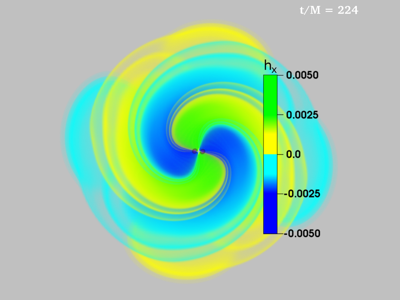
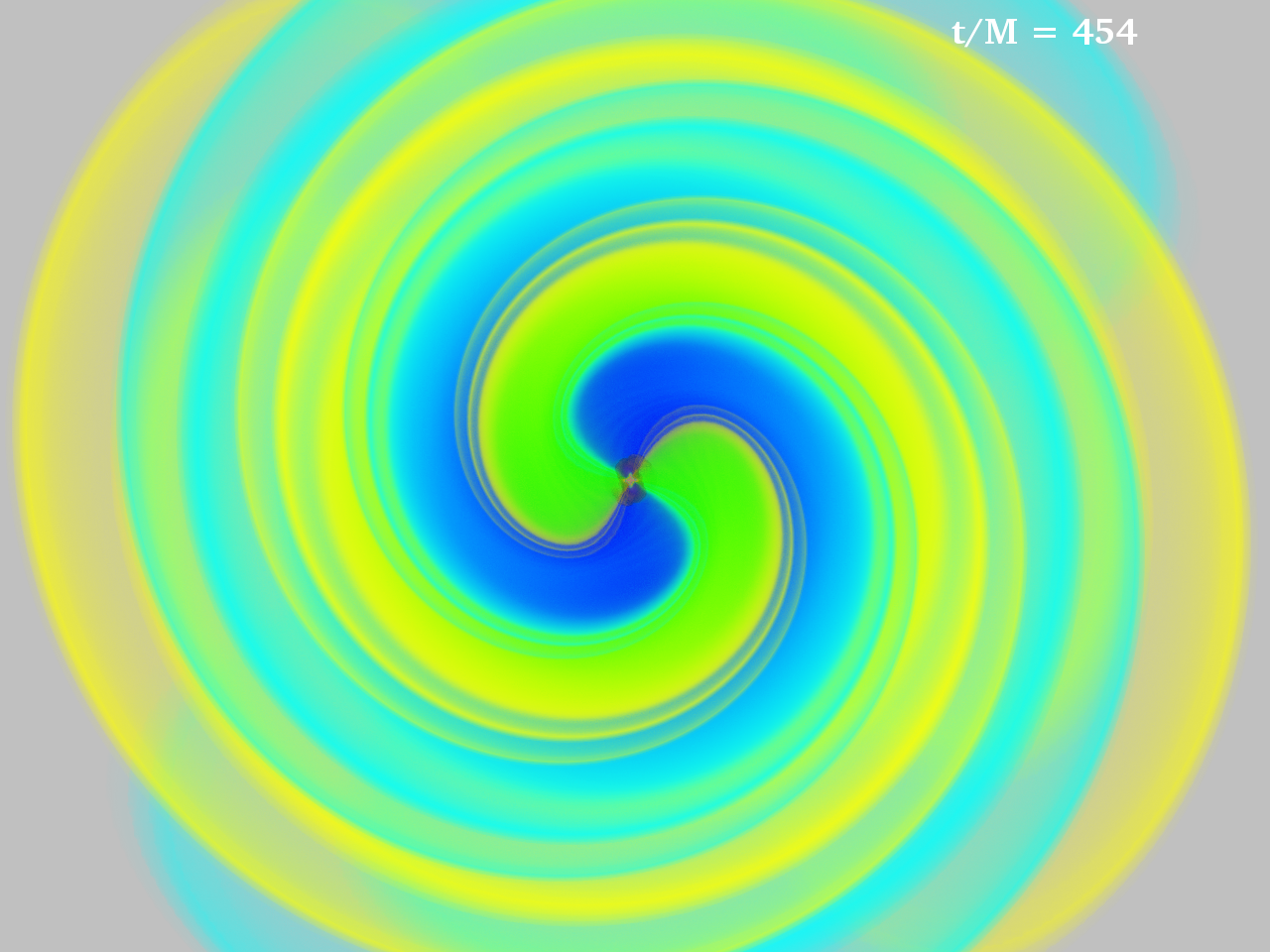
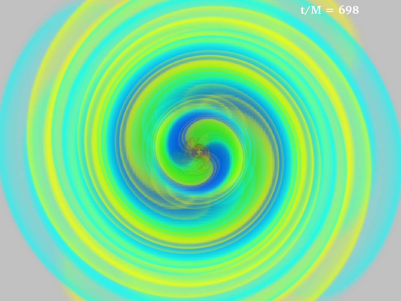
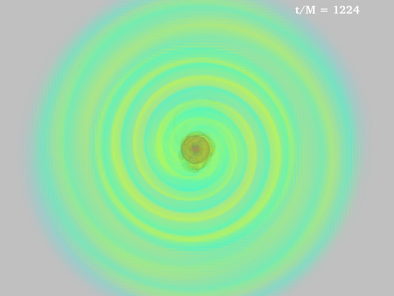
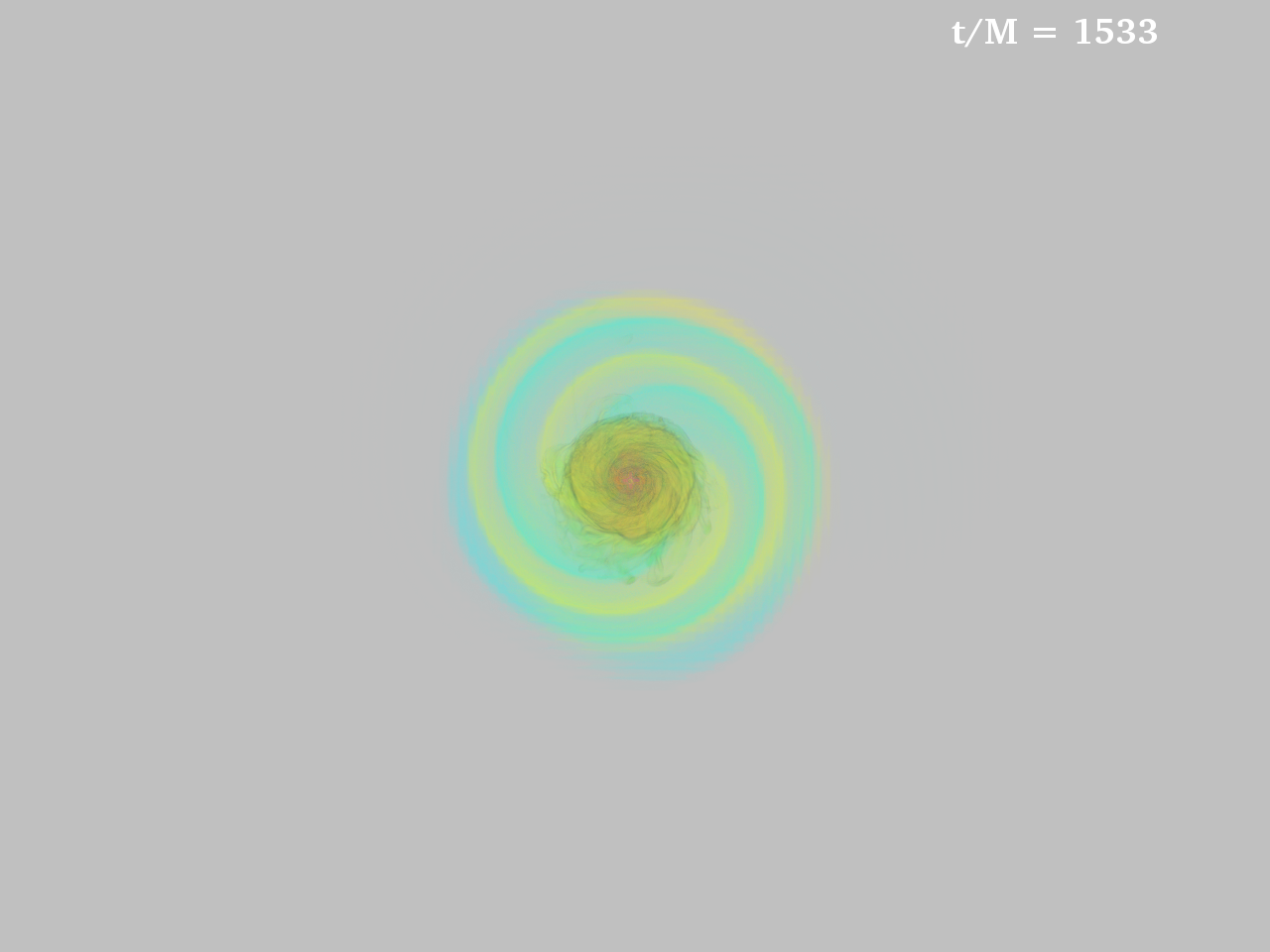
The gravitational wavetrain from an NSNS merger may be separated into four qualitatively different phases: the inspiral, merger, HMNS spindown and BH ringdown. During the inspiral phase, which takes up most of the binary's lifetime, gravity wave emission gradually reduces the binary separation. The merger phase of the gravitational wavetrain is characterized by tidal disruption of the neutron star, followed by the formation of a hypermassive neutron star (HMNS). As the HMNS spins down, it pulses and emits GWs. After the HMNS undergoes delayed collapse to a spinning BH, ringdown radiation is emitted as the distorted BH settles down to Kerr-like equilibrium (Note: Only in the case of a vacuum spacetime does the spinning BH obey the exact Kerr solution. The BHs formed here are surrounded by gaseous disks with small, but nonnegligible, rest mass). The h× polarization mode of the gravitational wave is shown below.
Waveform Analysis
Figure 2-1 shows the waveform of this case. The plot can be divided in three
regions. Region I is from $t/M = 0$ to $t/M \approx 580$, where the system is two neutron stars
orbiting each other. Region II is from $t/M\approx 580$ to $t/M \approx 1800$, where the system is a
hypermassive neutron star. Note that going from region I to region II,
the amplitude of the gravitational wave is decreased, and is slowly diminishing in time.
In region II, a weaker quadrupole wave is produced by the nonaxisymmetric spindown and pulsation of the HMNS.
Region III is from $t/M \approx 1800$ until the end. Here, the
amplitude goes to zero as the spinning BH rings downs.
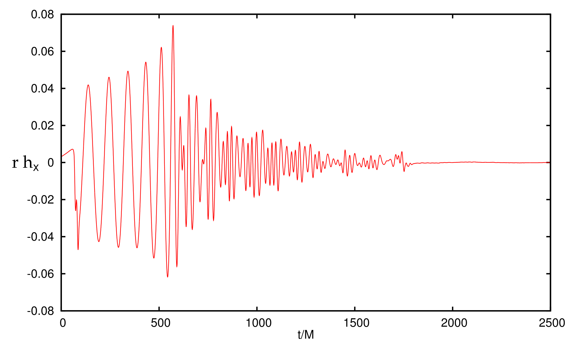
Fig 2-1: A plot of $h_{\times}$ vs. $t/M$ of the canonical interior+exterior NSNS case
Figure 2-2 shows the FFT of
Figure 2-1. Notice the peak at around $\Omega M = 0.07$.
This is the frequency of the gravitational wave in region I just prior to tidal breakup,
and it is indeed twice the orbital frequency of the neutron stars.
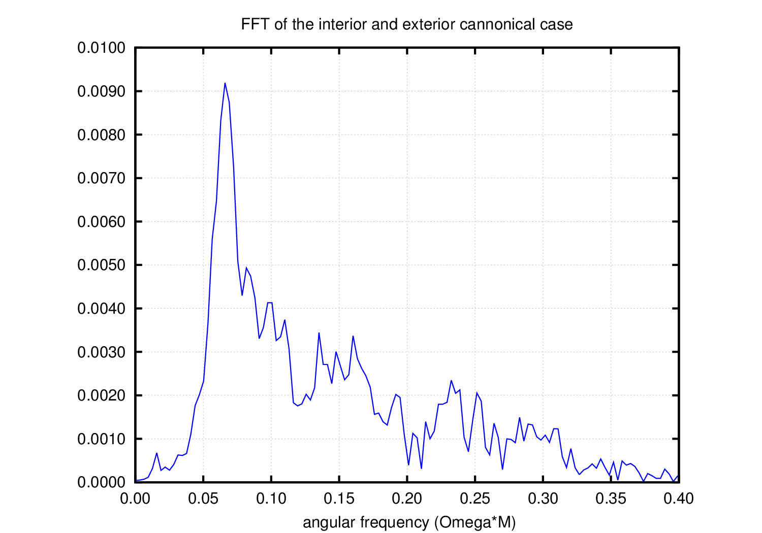
Fig 2-2: Fast Fourier transform of figure 2-1. The frequency is in units of
$\Omega M$.
In order to see the low frequency mode at the post-merger stage (Region II), we can FFT the waveform at times $t/M > 650$, and figure 2-3 is this plot.
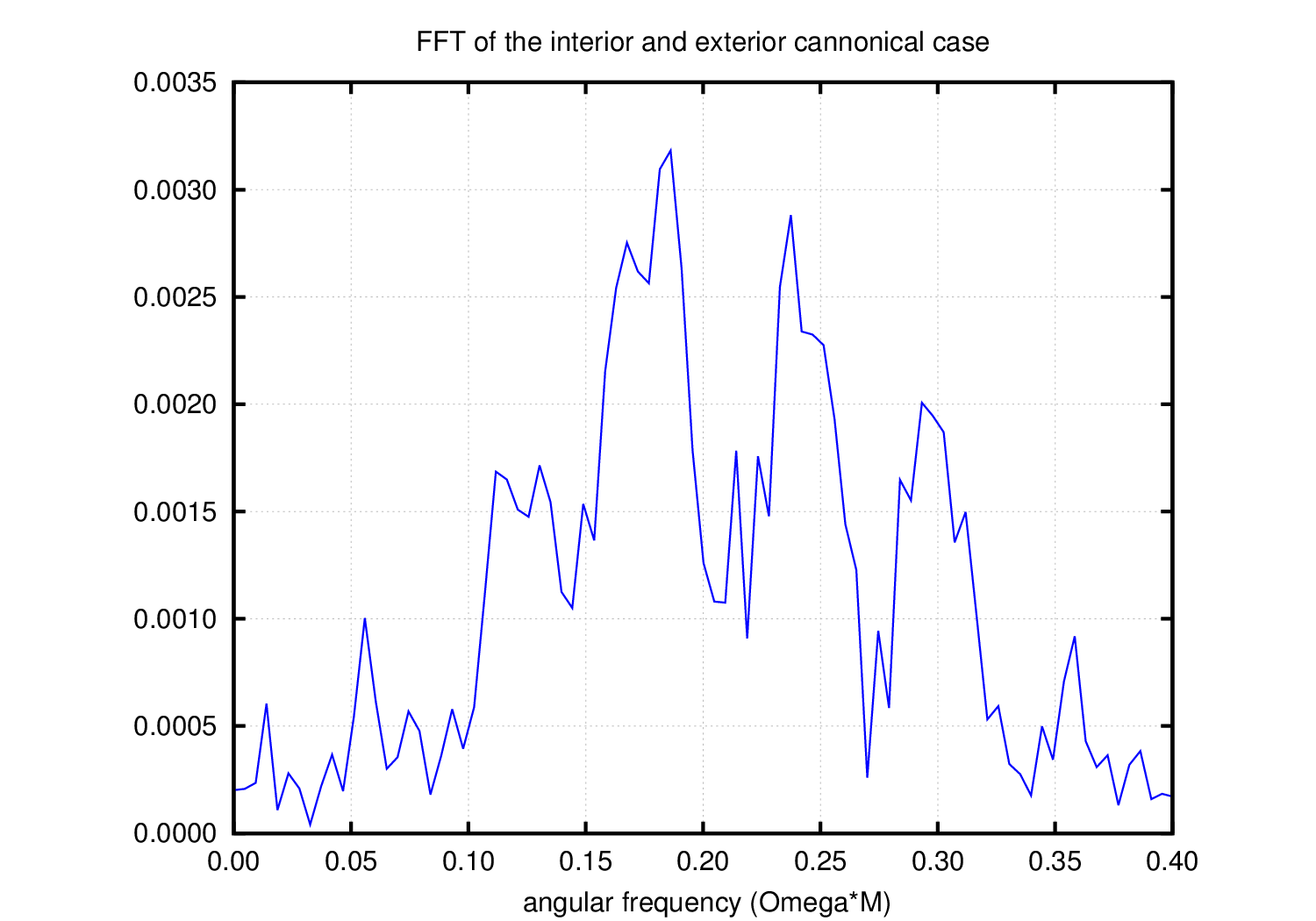
Fig 2-3: Fast Fourier transform of figure 2-1 for $t/M > 650$
Table 2-1 summarizes the computed frequencies in the NSNS system. $(\Omega M)_{GW}$ is the
peak-to-peak frequency of the gravitational wave, and $(\Omega M)_{orb}$ is the orbital angular
velocity of the NSNS binary, and $(\Omega M)_{GW-2}$ is the frequency of the secondary peaks in
region II of the figure 2-1. $(\Omega M)_{GW}$ is calculated in both region I, just prior to tidal
disruption, as well as in region II, just prior to HMNS delayed collapse. $(\Omega M)_{spin}$
is the spin angular velocity of non-axisymmetric HMNS just prior to delayed collapse. $(\Omega M)_{orb}$ and $(\Omega M)_{spin}$ are calculated by visually determing the
frequency in 3D movie. Note that in region I, $(\Omega M)_{GW} = 2(\Omega M)_{orb}$,
and in region II, $(\Omega M)_{GW} = 2(\Omega M)_{spin}$ as expected for quadrupole waves
| NSNS |
| $(\Omega M)_{GW} = 0.06628$ |
| $(\Omega M)_{orb} = 0.03396$ |
|
| HMNS |
| $(\Omega M)_{GW} = 0.18176$ |
| $(\Omega M)_{GW-2} = 0.05610$ |
| $(\Omega M)_{spin} = 0.08850$ |
|
Table 2-1: Table of frequency values for the interior and exterior canonical case.