Poynting Flux ("Lighthouse Effect")

1. Introduction
2. Initial Configuration
3. Case 1: S_BH/M_BH²=-0.5
4. Case 2: S_BH/M_BH²=0
5. Case 3: S_BH/M_BH²=0.75
6. Comparison

Introduction

Black hole-neutron star binaries are among the most promising sources for the simultaneous detection of gravitational wave and electromagnetic signals in the era of multimessenger astronomy. Apart from post-merger electromagnetic signals, detectable pre-merger signals may arise during a BHNS inspiral. Toward the end of the inspiral, strong magnetic fields will thread and sweep the black hole horizon, establishing a unipolar inductor (UI) DC circuit that extracts energy from the system. As these UIs operate in strongly curved, dynamical spacetimes, numerical relativity simulations are necessary to reliably determine the electromagnetic output. In addition to the UI luminosity, another important EM radiation mechanism that always operates here is that due to the accelerating magnetic dipole (MD) moment of the NS. MD emission dominates when UI does not operate, either because of corotation, or because it cannot be established due to the azimuthal twist of the magnetic flux tubes being too large, which may be the case for NSNS binaries. In all cases, the Poynting flux peaks within a broad beam of ~40^o in the azimuthal direction, and in the S_BH/M_BH²=0 and S_BH/M_BH²=0.75 cases within ~60^o from the orbital plane. This may establish a lighthouse effect as a characteristic EM signature of BHNS systems prior to merger, if the variation is not washed out by intervening matter.

Case 1: S_BH/M_BH²=-0.5

Here, we follow the evolution of the Poynting flux of a neutron star orbiting a spinning black hole, with S_BH/M_BH²=-0.5 (i.e., the BH spin angular momentum is antiparallel to the binary orbital angular momentum.) After a transient period caused by our choice of non-stationary initial magnetic fields, the luminosities settle to an approximately constant value as expected. We find a time-averaged luminosity after the first 1.5 orbits of

where B_NS,p is the NS polar magnetic field strength as measured by a CTS normal observer, and M_NS is the NS rest mass. As the magnetic field inside the NS does not affect the matter evolution, the EM luminosity scales exactly with B as indicated.

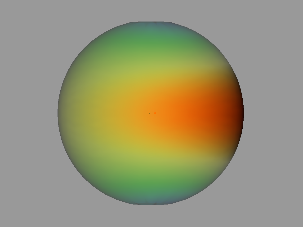Fig. 1-1: Poynting Flux at r = 120M at time t/M = 0	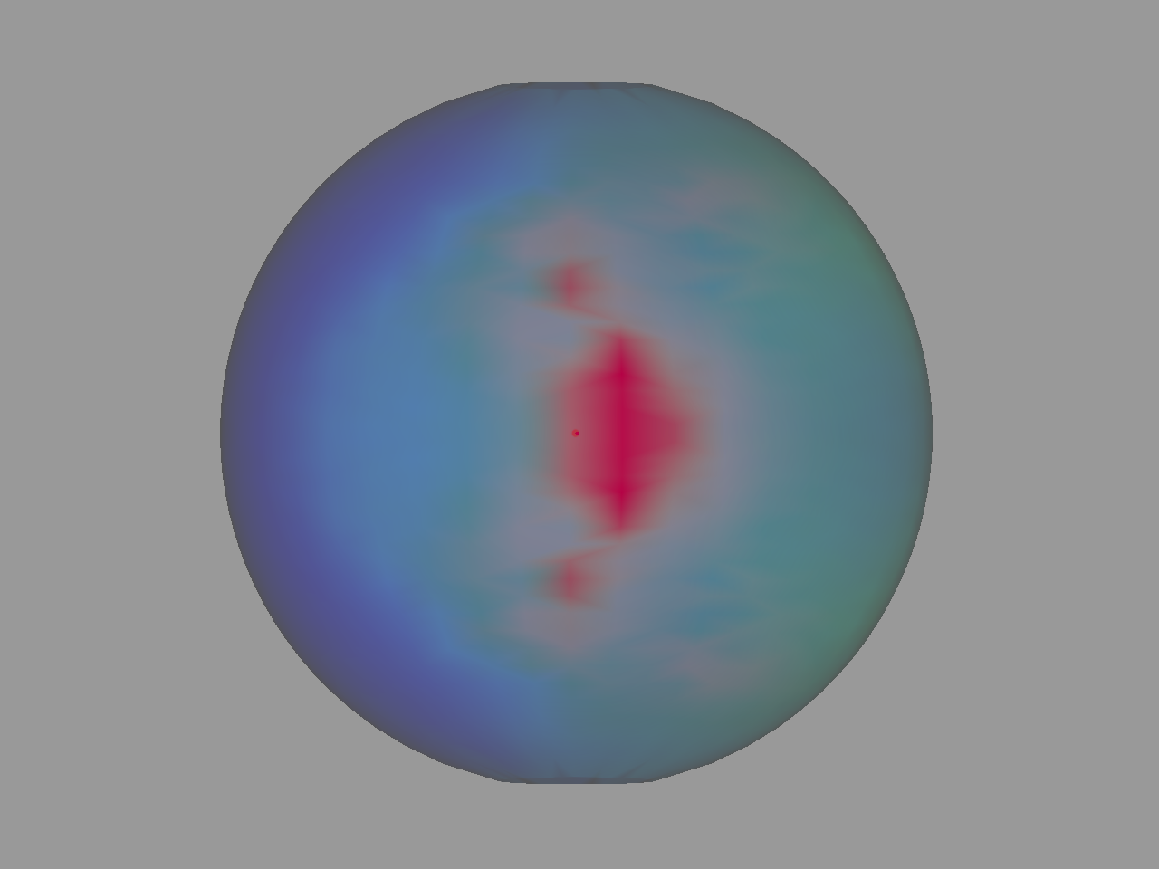Fig. 1-2: Poynting Flux at r = 120M at time t/M = 122
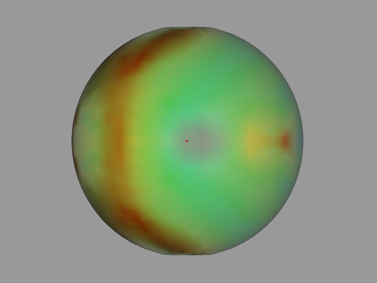Fig. 1-3: Poynting Flux at r = 120M at time t/M = 306	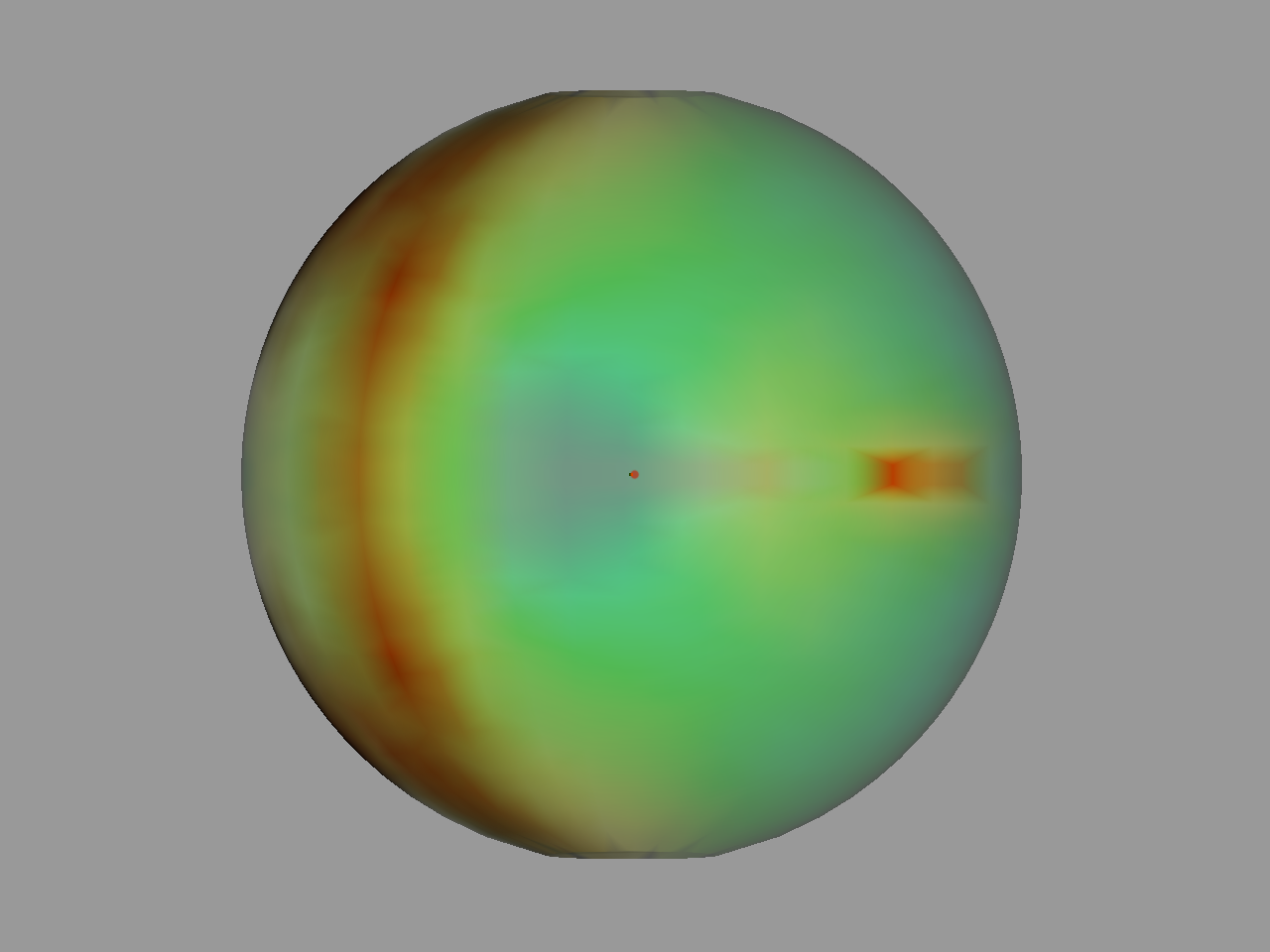Fig. 1-4: Poynting Flux at r = 120M at time t/M = 503

Case 2: S_BH/M_BH²=0

Here, we follow the evolution of the Poynting flux of a neutron star orbiting a nonspinning black hole. After a transient period caused by our choice of non-stationary initial magnetic fields, the luminosities settle to an approximately constant value as expected. We find a time-averaged luminosity after the first 1.5 orbits of

where B_NS,p is the NS polar magnetic field strength as measured by a CTS normal observer, and M_NS is the NS rest mass. As the magnetic field inside the NS does not affect the matter evolution, the EM luminosity scales exactly with B as indicated.

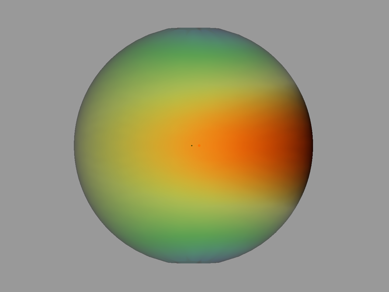Fig. 2-1: Poynting Flux at r = 120M at time t/M = 0	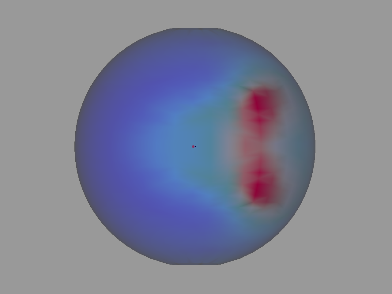Fig. 2-2: Poynting Flux at r = 120M at time t/M = 117
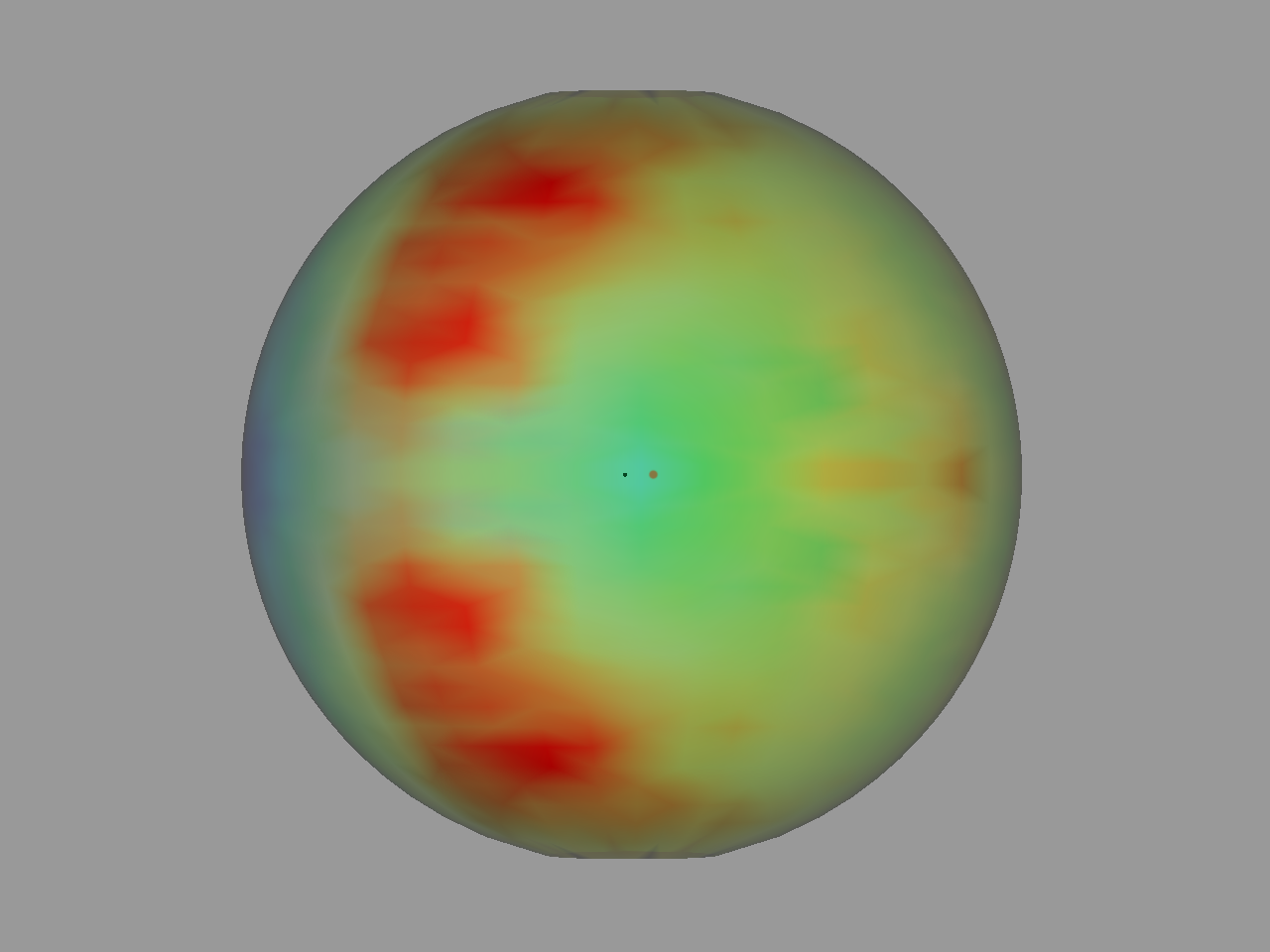Fig. 2-3: Poynting Flux at r = 120M at time t/M = 177	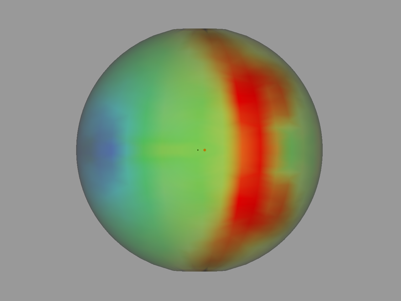Fig. 2-4: Poynting Flux at r = 120M at time t/M = 385

Case 3: S_BH/M_BH²=0.75

Here, we follow the evolution of the Poynting flux of a neutron star orbiting a spinning black hole, with S_BH/M_BH²=0.75 (i.e., the BH spin angular momentum is parallel to the binary orbital angular momentum.) After a transient period caused by our choice of non-stationary initial magnetic fields, the luminosities settle to an approximately constant value as expected. We find a time-averaged luminosity after the first 1.5 orbits of

where B_NS,p is the NS polar magnetic field strength as measured by a CTS normal observer, and M_NS is the NS rest mass. As the magnetic field inside the NS does not affect the matter evolution, the EM luminosity scales exactly with B as indicated.

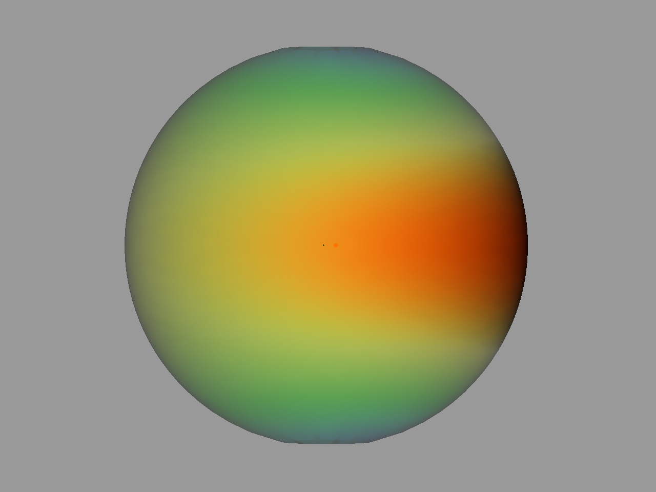Fig. 3-1: Poynting Flux at r = 120M at time t/M = 0	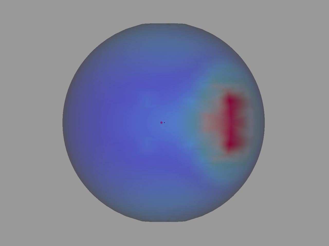Fig. 3-2: Poynting Flux at r = 120M at time t/M = 114
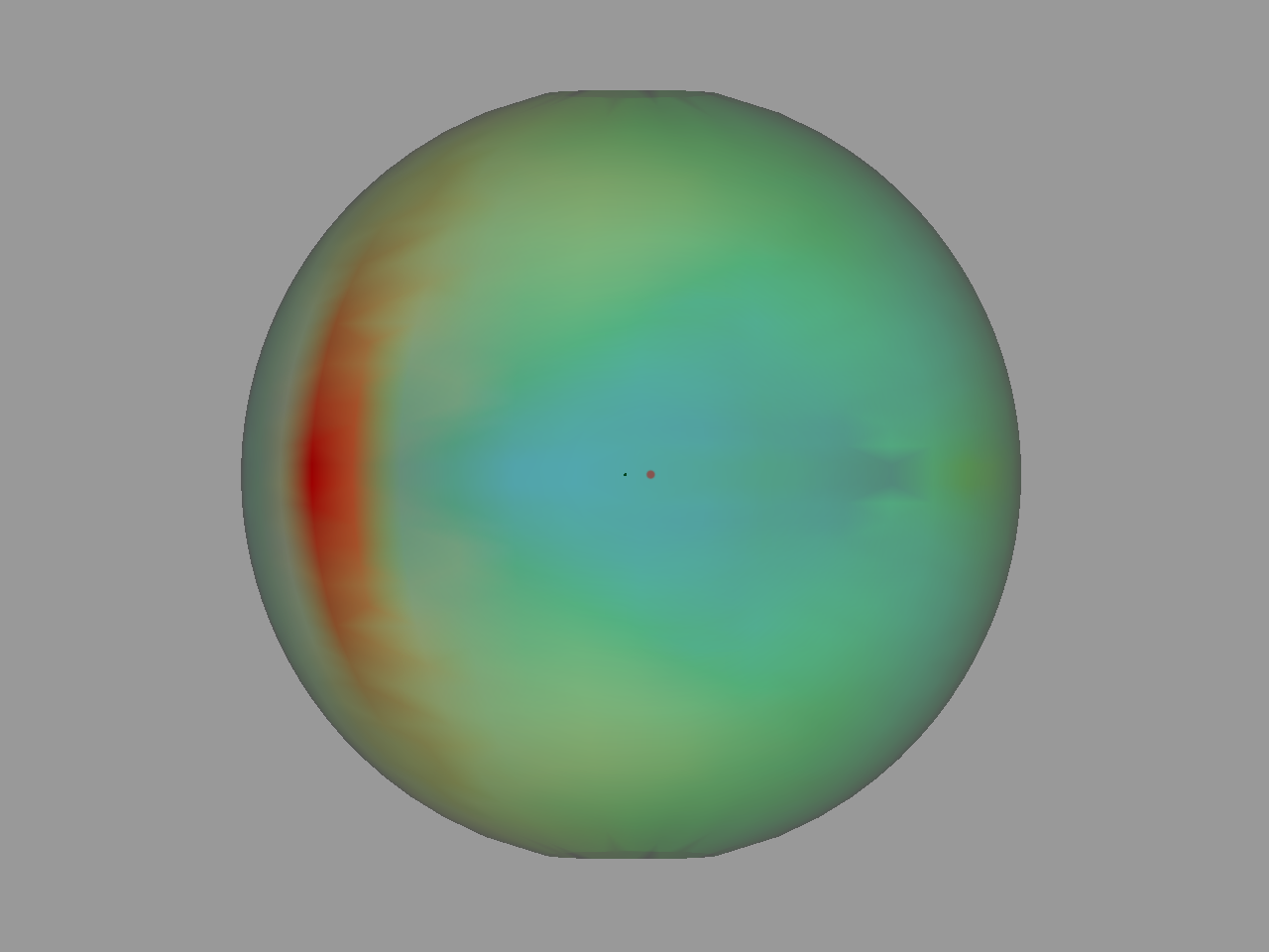Fig. 3-3: Poynting Flux at r = 120M at time t/M = 548	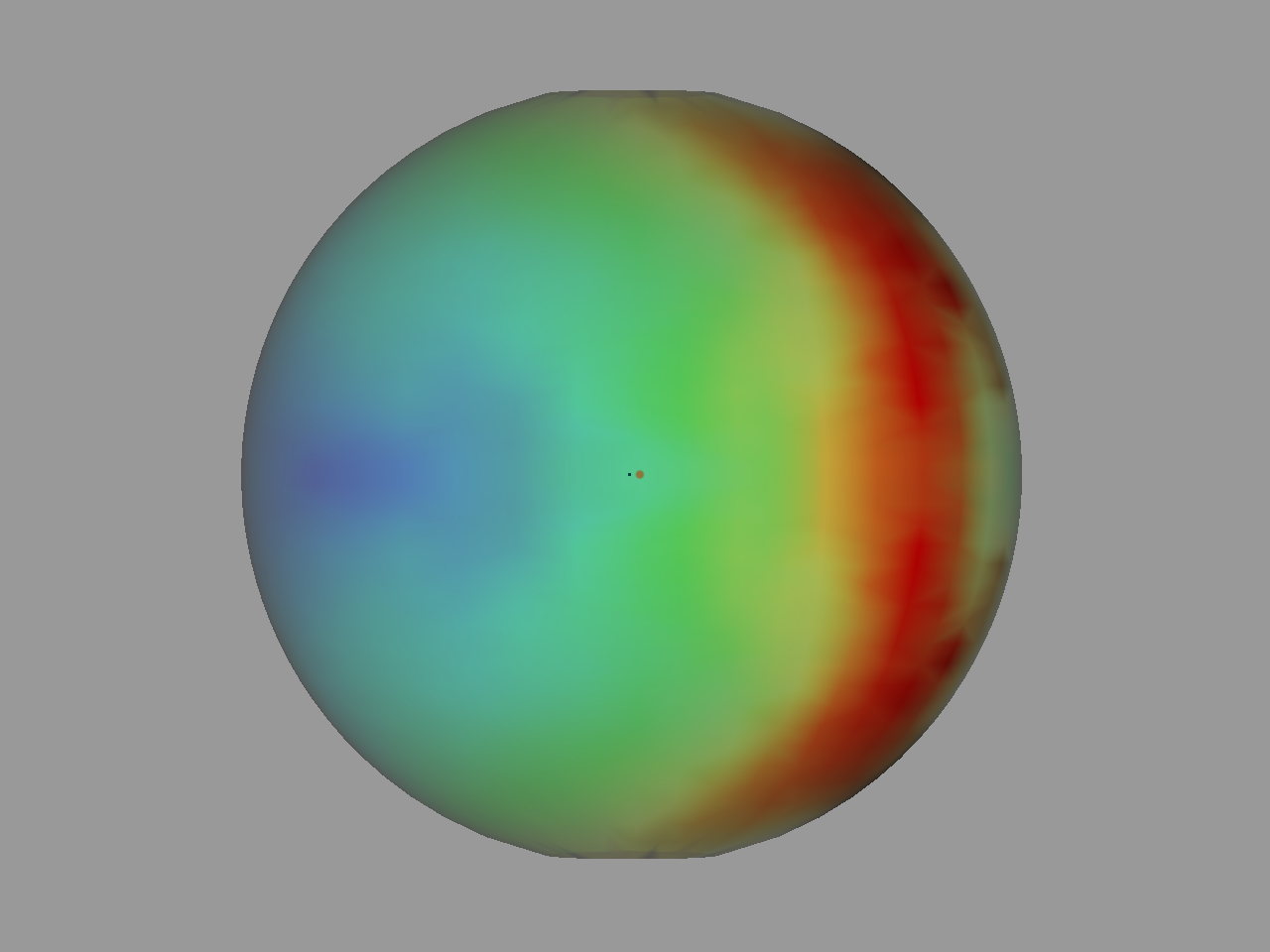Fig. 3-4: Poynting Flux at r = 120M at time t/M = 600

Comparison

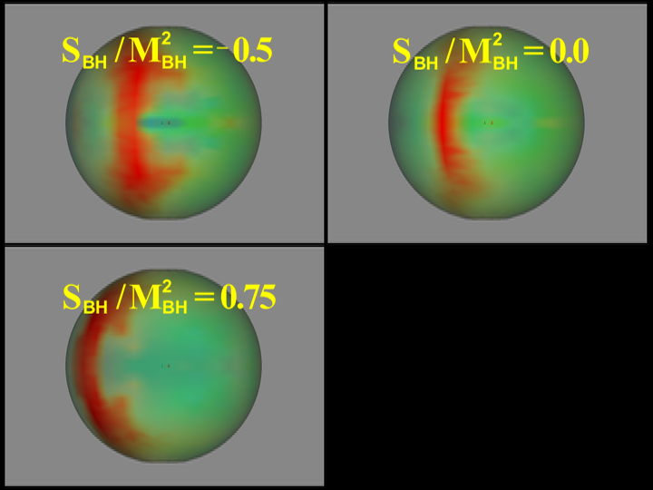Fig. 4-1: Poynting Flux at r = 120M at time t/M = 0	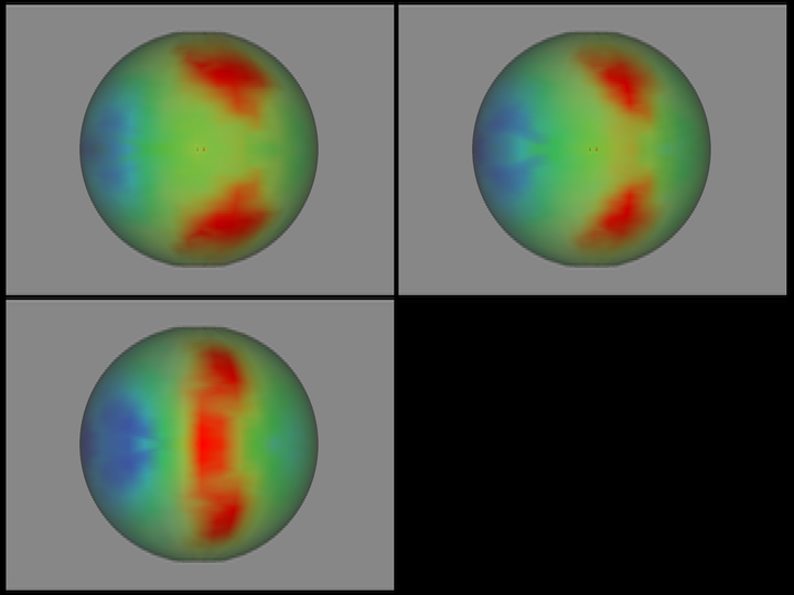Fig. 4-2: Poynting Flux at r = 120M at time t/M = 141
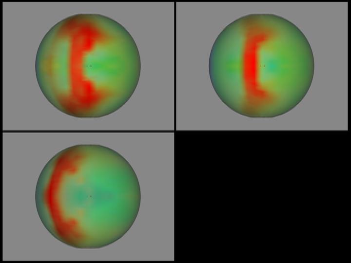Fig. 4-3: Poynting Flux at r = 120M at time t/M = 352	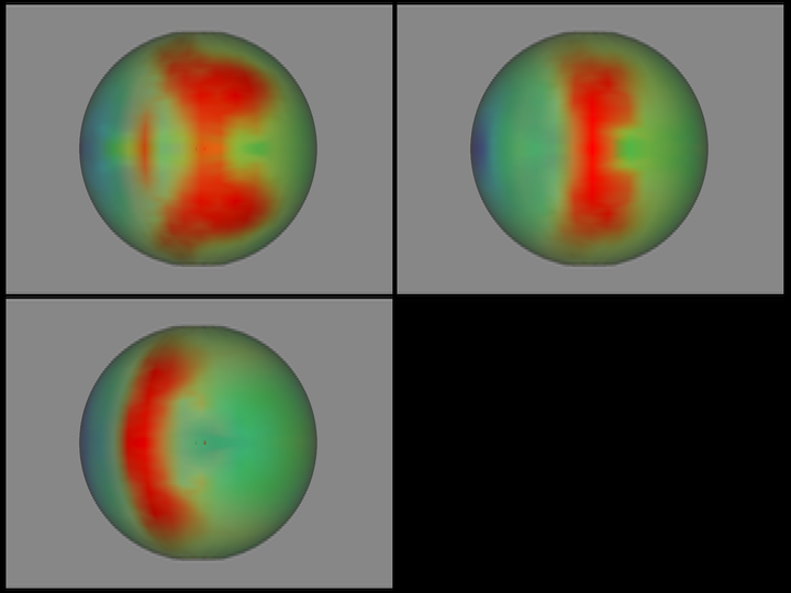Fig. 4-4: Poynting Flux at r = 120M at time t/M = 529