 r-Mode Movie

r-Mode Oscillations of Rotating Magnetic Neutron Stars
Frederick K. Lamb
Luciano Rezzolla
Stuart L. Shapiro
University of Illinois at Urbana-Champaign
Introduction: The Nature of r-Mode Oscillations
r-Mode oscillations in rotating neutron stars are an important topic of research in neutron star stability. r-Modes, also called Rossby waves, are unstable in any arbitrarily slowly rotating star if one assumes a perfect fluid and no magnetic field. Gravitational radiation causes this instability. The r-mode amplitude increases because the angular momentum gravity waves carry away is negative. In a perfect fluid, the r-mode amplitude becomes unbounded. In effect, neutron stars undergoing r-mode oscillations are potentially a strong source of gravitational radiation. In the following animations, we illustrate the properties of r-modes and how they might interact with stellar magnetic fields.
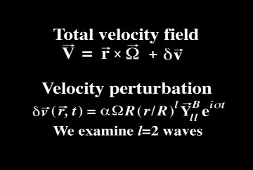
The perturbation to rotational motion is the lowest-order Newtonian velocity perturbation. It is produced by small-amplitude r-mode oscillations of a slowly and uniformly rotating, nonmagnetic, inviscid, fluid star. Here, we take l = 2 and consider only the terms linear in a, the dimensionless amplitude.
Scene 1: Velocity Perturbations as Seen in the r-Mode Pattern Frame
Download Quicktime (5.0 Mb)
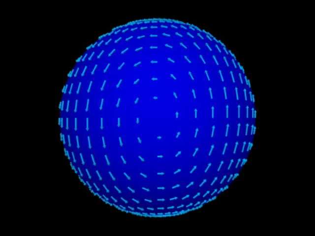
In this movie we show the r-mode velocity perturbation, dv, as seen in the pattern frame. We show velocity vectors at points on the star's surface in light blue. We rotate the observer around the star. In the pattern frame, the velocity perturbation is time independent. The dimensionless amplitude a = 0.3.
Scene 2: Total Velocity Field and Fluid Motion as Seen in the r-Mode Pattern Frame
Download Quicktime (6.8 Mb)
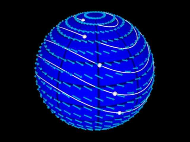
We now consider particle motion in the pattern frame. White dots represent massless pointlike fluid elements, and we use the dark grid to illustrate the rotation of the unperturbed fluid in this frame. To evolve the fluid elements we must consider the rotation of the star relative to this frame. The new velocity vectors reflect the addition of rotational velocity. Note that particle trajectories are closed. Again, a = 0.3.
Download Quicktime (5.3 Mb)
We then rotate the observer around the star to see its full character.
Scene 3: Velocity Field and Fluid Motion as Seen in the Corotating Frame
Download Quicktime (8.6 Mb)
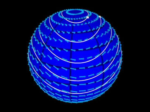
We change frames to the corotating frame. The dark grid, which represents the unperturbed fluid, remains stationary in this frame. In this animation we first rotate the observer up from the equatorial plane. Then we follow particle trajectories and time evolve the velocity vectors in the corotating frame. One should note that there is oscillatory motion as well as secular drift. Secular drift is actually a second-order effect that arises when one integrates the first-order equations. The dimensionless amplitude a = 0.3.
Scene 4: Fluid Motion as Seen in the Inertial Frame
Download Quicktime (6.3 Mb)
The observer is now in an inertial frame (one that is not rotating about the star at all). We follow particles as they rotate with the star and undergo small perturbations. The dark grid shows the rotation of the star, and white trails represent particle trajectories. Here, a = 0.15.
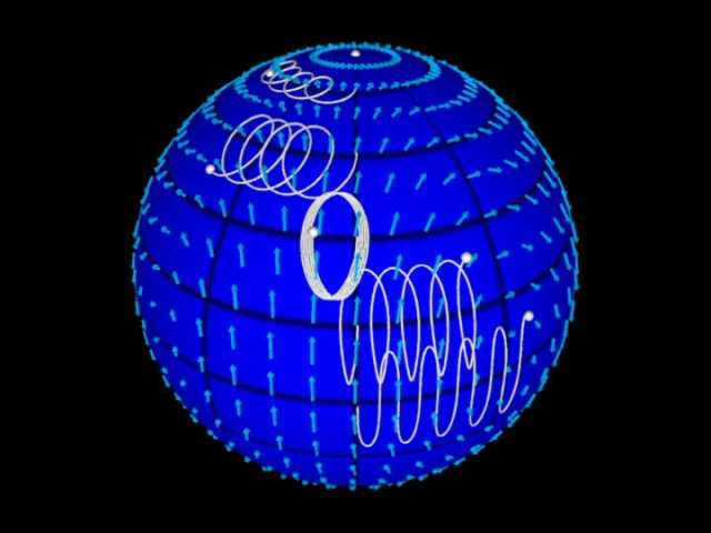
Scene 5: Distortion of a Magnetic Field Line as Seen in the Corotating Frame
The field line we consider initially connects particles along a meridian of the star. The field line is yellow, and a few of the particles that the field line intersects are shown in white.
Download Quicktime (3.9 Mb)
We then time evolve the magnetic field line. The new field line is shown in yellow and has become appreciably distorted. The field line distortion results from the secular drift of the particles. We neglect any back-reaction of the magnetic field and assume that the field line is tied to the perfectly conducting fluid elements. Thus, we utilize the magnetohydrodynamic (MHD) approximation. In effect, we follow the particles that made up the initial field line and connect them to generate the new field line as time progresses. The trails of a few of the particles are shown in white. a = 0.3.
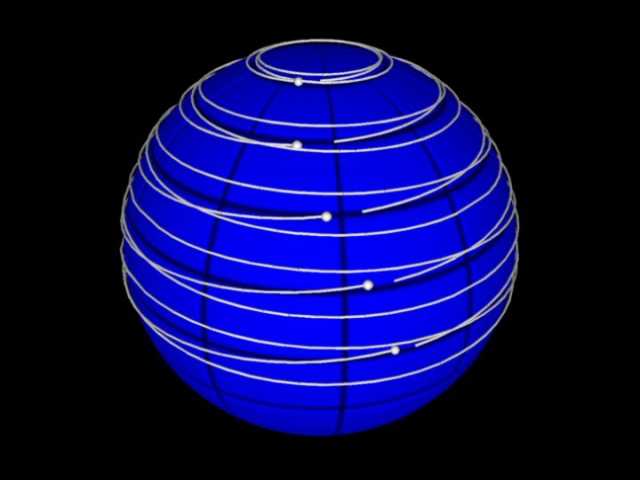
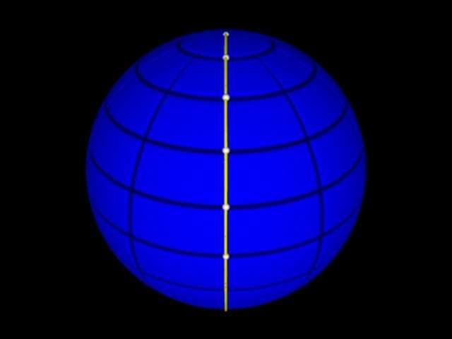
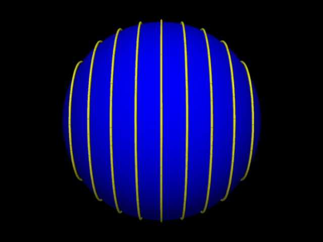
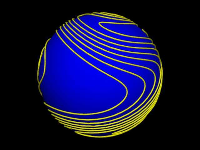
Scene 6: Distortion of a Set of Magnetic Field Lines as Seen in the Corotating Frame
Download Quicktime (2.1 Mb)
Now, we consider a set of field lines. They lie on the surface and circle the star. We rotate the observer around the star to see the field's full character.
Download Quicktime (21.2 Mb)
We then time evolve the field lines using the MHD approximation as in the movie above. The field lines are initially straight but soon become distorted and crowded together. a = 0.3.
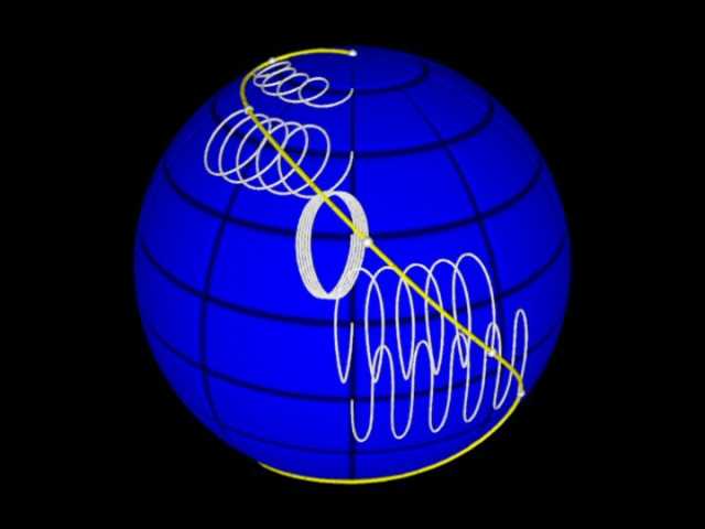
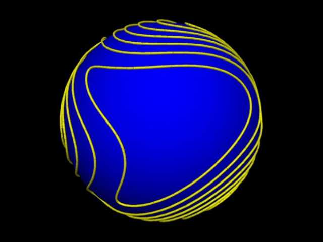
Scene 7: Distortion of a Set of Magnetic Field Lines as Seen in the Inertial Frame
Download Quicktime (24.4 Mb)
This situation has the the same initial conditions as the previous movie. Now, the observer is in the inertial frame. Also, we reduce the speed of the movie by one third to better show the evolution of the field lines.
Scientific visualization by
Harish Agarwal
Randall Cooper
Bradley Hagan
Patrick McGrath
Jared Mehl
David Webber
Undergraduate Research Team
Departments of Physics and Astronomy
University of Illinois at Urbana-Champaign
last updated 6/27/02 by rlc